Orbital Angular Momentum in Quantum Mechanics
Daniel Fischer
From Quantum Mechanics to the Atom
We now have most of the mathematical tools we need.
The next challenge is to apply them to a real physical system:
How do we describe an atom quantum mechanically?
1. The Hydrogen Atom
Consider the simplest atom:
- one proton
- one electron
- interacting through the Coulomb force
What do we want to know?
We want to find the stationary quantum states of the system, i.e. states with a well-defined energy.
1.1 Stationary States
In abstract notation, stationary states satisfy the energy eigenvalue equation
\[ \hat H |\psi\rangle = E |\psi\rangle. \]
This is the time-independent Schrödinger equation (TISE).
The problem is therefore:
Find the eigenstates and eigenvalues of the Hamiltonian.
But how do we actually solve this equation?
1.2 Choose a Representation
To solve the problem explicitly, we choose the coordinate representation.
The state becomes a wave function
\[ \Psi(\mathbf r_e,\mathbf r_p) = \langle \mathbf r_e,\mathbf r_p|\psi\rangle. \]
The Hamiltonian contains the kinetic energies of both particles and their Coulomb interaction:
\[ \left[ -\frac{\hbar^2}{2m_e}\nabla_e^2 -\frac{\hbar^2}{2m_p}\nabla_p^2 -\frac{e^2}{4\pi\epsilon_0|\mathbf r_e-\mathbf r_p|} \right] \Psi(\mathbf r_e,\mathbf r_p) = E\Psi(\mathbf r_e,\mathbf r_p). \]
1.3 A Six-Dimensional Problem
The wave function depends on
\[ \mathbf r_e=(x_e,y_e,z_e), \qquad \mathbf r_p=(x_p,y_p,z_p). \]
So, as written, this is a six-dimensional differential equation.
Fortunately, much of this motion is physically trivial.
2. Center-of-Mass and Relative Motion
Introduce the center-of-mass coordinate
\[ \mathbf R = \frac{m_e\mathbf r_e+m_p\mathbf r_p}{m_e+m_p} \]
and the relative coordinate
\[ \mathbf r=\mathbf r_e-\mathbf r_p. \]
The Hamiltonian separates into
\[ \hat H=\hat H_{\rm CM}+\hat H_{\rm rel}. \]
2.1 Internal Motion
The center of mass describes the free translation of the atom as a whole.
For atomic structure, we are interested in the internal motion.
The relative-motion Hamiltonian is
\[ \hat H_{\rm rel} = -\frac{\hbar^2}{2\mu}\nabla^2 -\frac{e^2}{4\pi\epsilon_0 r}, \]
where
\[ \mu=\frac{m_e m_p}{m_e+m_p} \]
is the reduced mass.
Thus we need to solve
\[ \left[ -\frac{\hbar^2}{2\mu}\nabla^2 +V(r) \right] \psi(\mathbf r) = E\psi(\mathbf r). \]
3. The Importance of Symmetry
For the Coulomb interaction,
\[ V(r) = -\frac{e^2}{4\pi\epsilon_0 r}. \]
The potential depends only on the distance between proton and electron.
It does not depend on the direction of \(\mathbf r\).
This has two major consequences.
3.1 Consequence 1: Spherical Coordinates
Because the potential depends only on
\[ r=|\mathbf r|, \]
the problem has spherical symmetry.
Cartesian coordinates are therefore not the most natural choice.
We will ultimately use
\[ (r,\theta,\phi). \]
Keep this in mind — we will come back to it when we solve the hydrogen wave function.
3.2 Consequence 2: Angular Momentum
A central potential is invariant under rotations.
Rotational symmetry implies conservation of angular momentum.
In quantum mechanics, this means
\[ [\hat H,\hat{\mathbf L}]=0. \]
In particular,
\[ [\hat H,\hat L^2]=0, \qquad [\hat H,\hat L_z]=0. \]
So before we can solve the hydrogen atom, we need to understand orbital angular momentum in quantum mechanics.
4. Orbital Angular Momentum
From here: blackboard derivation
Classically,
\[ \mathbf L=\mathbf r\times\mathbf p. \]
In quantum mechanics,
\[ \hat{\mathbf L} = \hat{\mathbf r}\times\hat{\mathbf p}. \]
4.1 Angular Momentum Operators
In the coordinate representation,
\[ \hat{\mathbf p}=-i\hbar\nabla. \]
For example,
\[ \hat L_z = \hat x\hat p_y-\hat y\hat p_x \]
becomes
\[ \hat L_z = -i\hbar \left( x\frac{\partial}{\partial y} - y\frac{\partial}{\partial x} \right). \]
The other components follow by cyclic permutation.
4.2 Commutation Relations
The Cartesian components satisfy
\[ [\hat L_x,\hat L_y] = i\hbar\hat L_z, \]
with cyclic permutations.
Therefore,
\[ [\hat L_x,\hat L_y]\neq 0. \]
The components of angular momentum cannot, in general, all have simultaneously well-defined values.
This connects directly to our discussion of measurement and uncertainty.
4.3 Total Angular Momentum
Define
\[ \hat L^2 = \hat L_x^2+\hat L_y^2+\hat L_z^2. \]
Unlike the individual components,
\[ [\hat L^2,\hat L_z]=0. \]
So we can look for simultaneous eigenstates of \(\hat L^2\) and \(\hat L_z\):
\[ \hat L^2|\ell,m\rangle = \lambda|\ell,m\rangle, \]
\[ \hat L_z|\ell,m\rangle = \mu|\ell,m\rangle. \]
4.4 Angular Momentum in Spherical Coordinates
Using
\[ x=r\sin\theta\cos\phi, \qquad y=r\sin\theta\sin\phi, \qquad z=r\cos\theta, \]
one finds
\[ \hat L_z = -i\hbar\frac{\partial}{\partial\phi}. \]
The important point is that \(\hat L_z\) acts only on the azimuthal coordinate \(\phi\).
4.5 The \(L_z\) Eigenvalue Problem
Consider
\[ \hat L_z \Phi(\phi)=\mu\Phi(\phi). \]
Using
\[ \hat L_z = -i\hbar\frac{\partial}{\partial\phi}, \]
we obtain
\[ -i\hbar\frac{d\Phi}{d\phi} = \mu\Phi. \]
The solution is
\[ \Phi(\phi)=A e^{i\mu\phi/\hbar}. \]
4.6 Quantization of \(L_z\)
The wave function must be single-valued:
\[ \Phi(\phi+2\pi)=\Phi(\phi). \]
Therefore,
\[ e^{i2\pi\mu/\hbar}=1. \]
This requires
\[ \mu=m\hbar, \qquad m\in\mathbb Z. \]
Hence
\[ \boxed{L_z=m\hbar}. \]
4.7 The Remaining Angular Equation
Solving the full angular problem gives the spherical harmonics
\[ Y_\ell^m(\theta,\phi). \]
They satisfy
\[ \hat L^2Y_\ell^m = \hbar^2\ell(\ell+1)Y_\ell^m, \]
and
\[ \hat L_zY_\ell^m = m\hbar Y_\ell^m. \]
The allowed quantum numbers are
\[ \ell=0,1,2,\ldots \]
and
\[ m=-\ell,-\ell+1,\ldots,\ell. \]
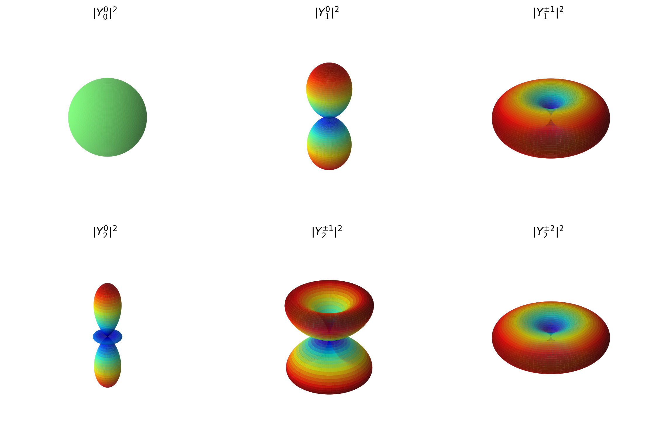
5. Spherical Harmonics
For the lowest values of \(\ell\) and \(m\):
\[ Y_0^0 = \sqrt{\frac{1}{4\pi}}, \qquad Y_1^0 = \sqrt{\frac{3}{4\pi}}\cos\theta, \]
\[ Y_1^{\pm1} = \mp\sqrt{\frac{3}{8\pi}}\sin\theta\,e^{\pm i\phi}. \]
These functions describe the angular part of the atomic wave function.
5.1 Graphical Representation
6. What Have We Learned?
Orbital angular momentum is quantized:
\[ \boxed{ L^2=\hbar^2\ell(\ell+1) } \]
and
\[ \boxed{ L_z=m\hbar } \]
with
\[ \ell=0,1,2,\ldots, \qquad m=-\ell,\ldots,\ell. \]
6.1 Back to the Hydrogen Atom
We started with
\[ \left[ -\frac{\hbar^2}{2\mu}\nabla^2+V(r) \right]\psi(\mathbf r) = E\psi(\mathbf r). \]
Because the Coulomb potential is spherically symmetric, the wave function can be organized according to the angular-momentum quantum numbers \(\ell\) and \(m\).
The angular dependence is described by
\[ Y_\ell^m(\theta,\phi). \]
What remains is the radial part of the hydrogen problem.
7. Key Takeaways
- The hydrogen atom is a two-body quantum problem.
- Center-of-mass motion separates from the internal motion.
- The Coulomb potential depends only on \(r\), so the system is rotationally symmetric.
- Rotational symmetry makes angular momentum a conserved quantity.
- \(\hat L^2\) and \(\hat L_z\) can be simultaneously diagonalized.
- Their eigenvalues are
\[ L^2=\hbar^2\ell(\ell+1), \qquad L_z=m\hbar. \]
- The corresponding angular wave functions are the spherical harmonics \(Y_\ell^m(\theta,\phi)\).
Additional Notes: Ladder Operators
The ladder operators are defined by
\[ L_\pm=L_x\pm iL_y. \]
They change the magnetic quantum number:
\[ L_\pm|\ell,m\rangle = \hbar \sqrt{ \ell(\ell+1)-m(m\pm1) } |\ell,m\pm1\rangle. \]
Thus \(L_+\) raises \(m\) and \(L_-\) lowers \(m\).
Additional Notes: Dirac Notation
The abstract angular-momentum states are related to their coordinate-space representation by
\[ \langle \theta,\phi|\ell,m\rangle = Y_\ell^m(\theta,\phi). \]
They are orthonormal:
\[ \langle \ell,m|\ell',m'\rangle = \delta_{\ell\ell'}\delta_{mm'}. \]
And satisfy
\[ \hat L^2|\ell,m\rangle = \hbar^2\ell(\ell+1)|\ell,m\rangle, \]
\[ \hat L_z|\ell,m\rangle = \hbar m|\ell,m\rangle. \]