Electron Spin and Fine Structure

Electron Spin and Fine Structure: Overview and Plan

This chapter introduces the concept of electron spin and its consequences for the energy structure of atoms, particularly the hydrogen atom. We discuss how spin interacts with orbital angular momentum to produce fine structure in atomic spectra and how relativistic corrections refine the energy levels.

The specific goals for this chapter are:

1. Introduce the electron spin operator \(\hat{\vec S}\), its eigenvalues, and its commutation relations, highlighting the analogy to orbital angular momentum.
2. Present the Pauli matrix representation of spin-\(\tfrac{1}{2}\) systems and demonstrate explicitly the commutator relations and eigenvalue equations.
3. Describe how the spin of the electron is combined with orbital angular momentum to define the total angular momentum \(\hat{\vec J} = \hat{\vec L} + \hat{\vec S}\).
4. Derive the form of the spin–orbit interaction in the Hamiltonian and show how it modifies the conserved quantum numbers.
5. Explain how the new complete set of quantum numbers \(|n, \ell, s, j, m_j\rangle\) is constructed using Clebsch–Gordan coefficients and the concept of the identity operator in a complete basis.
6. Discuss the fine-structure energy shifts, their origin from spin–orbit coupling and relativistic corrections, and the connection to the Dirac equation results.
7. Introduce term symbols (\({ }^{2S+1}L_J\)) and their use in describing atomic states, including the labeling of fine-structure-split energy levels.

By the end of this chapter, the student should be able to describe the spin of the electron, understand its contribution to the fine structure of atomic spectra, and connect the quantum numbers of total angular momentum to the observed energy level splittings.

---

1. Historical Pretext

Before introducing the modern concept of electron spin, it is useful to recall two classic experiments that shaped our understanding of angular momentum and magnetic moments in atoms: the Stern–Gerlach experiment (1922) and the Einstein–de Haas experiment (1915).

These experiments predate the explicit formulation of electron spin, and neither was originally interpreted in terms of spin. Nevertheless, they demonstrated crucial features of angular momentum quantization and the connection between angular momentum and magnetism.

1.1 The Stern–Gerlach Experiment

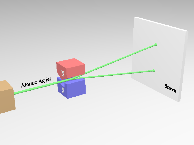
In 1922, Otto Stern and Walther Gerlach sent a beam of neutral silver atoms through an inhomogeneous magnetic field (Stern & Gerlach, 1922).

• Setup: A heated oven produces a jet of silver atoms, which is then collimated into a narrow beam. The beam enters a region between specially shaped magnet poles, arranged so that the magnetic field is not uniform but has a strong vertical gradient.
  
• After passing through the magnet, the atoms travel to a distant detection screen, where their spatial distribution can be recorded.

What happens physically?
The silver atom has a single unpaired electron, whose magnetic moment interacts with the field gradient. Classically, one would expect a continuous spread of deflections depending on the orientation of the magnetic moment. Instead, the beam splits cleanly into two spots on the screen. This demonstrates that the angular momentum component along the field axis can take only discrete values — the phenomenon of spatial quantization (Richtungsquantelung).

Stern–Gerlach experiment: an atomic beam is split into two distinct components by the inhomogeneous magnetic field, showing discrete orientations of angular momentum. Important components: atomic beam source (left), magnet with N/S poles (center), and detection screen (right).

---

1.2 The Einstein–de Haas Experiment

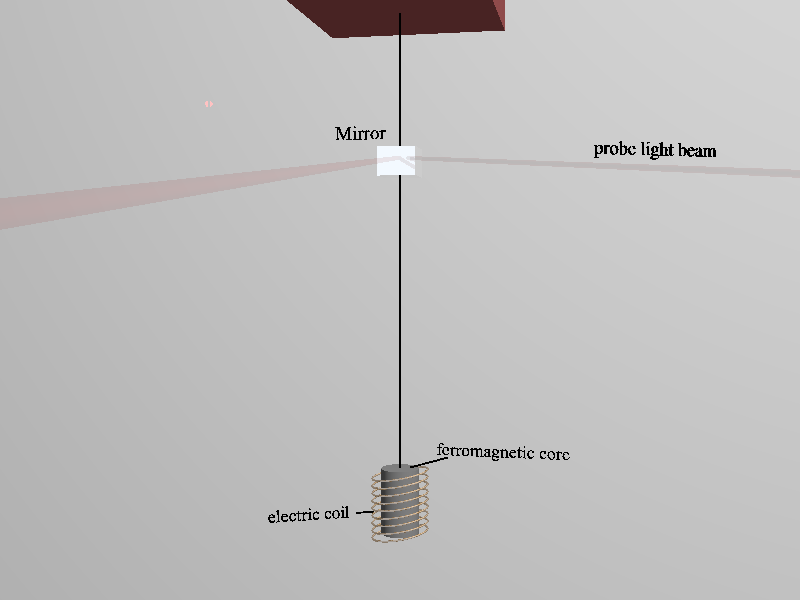
Several years earlier, in 1915, Albert Einstein and Wander Johannes de Haas performed an elegant experiment demonstrating the intimate relation between magnetism and angular momentum (Einstein & de Haas, 1915).

• Setup: A ferromagnetic cylinder (often iron) is suspended by a thin fiber, allowing it to rotate freely about its vertical axis.
  
• Around the cylinder is a coil of wire wound on a ferromagnetic core.
  
• When a current is switched on in the coil, it changes the magnetization of the cylinder.
  
• A small mirror is attached to the suspension, so that the mechanical rotation of the cylinder can be detected optically using a reflected probe light beam.

What happens physically?
When the magnetization of the cylinder is reversed, its internal electron magnetic moments flip orientation. Because each magnetic moment is associated with angular momentum, conservation of angular momentum requires the cylinder itself to rotate in the opposite direction. The effect is small but measurable, and the mirror–light setup amplifies the detection. The experiment showed that magnetization arises from angular momentum. However, the ratio of magnetic moment to angular momentum was found to differ by a factor of two from classical expectations — a puzzle later resolved by the discovery of electron spin.

Einstein–de Haas experiment: reversing the magnetization of a suspended ferromagnetic cylinder induces mechanical rotation, detected via a mirror and probe light. Important components: suspended cylinder, surrounding coil, ferromagnetic core, and optical detection system.

---

1.3 Historical Perspective

At the time of their original publication, neither the Stern–Gerlach nor the Einstein–de Haas experiment was interpreted in terms of an intrinsic electron spin — the very concept did not yet exist. Instead, both were framed within the language of orbital angular momentum and the then-prevailing Bohr–Sommerfeld model of the atom.

The Stern–Gerlach experiment

Stern and Gerlach themselves interpreted their observation of beam splitting as evidence for the quantization of orbital angular momentum along the field axis (“Richtungsquantelung”). Within the Bohr–Sommerfeld picture, an electron orbiting in a quantized elliptical trajectory would carry an orbital magnetic moment. Measuring its projection along the \(z\)-axis should then yield discrete values, consistent with their result.

What is striking in hindsight is that the silver atom has only a single valence electron in an \(s\)-orbital (\(\ell = 0\)). The Schrödinger wave mechanics (formulated a few years later, in 1926) would predict no orbital magnetic moment at all in this case, and thus no splitting. Yet Stern and Gerlach observed two distinct components, not more and not less.

This outcome was “accidentally” consistent with the Bohr–Sommerfeld model, which predicted two possible orientations for the angular momentum in this situation, but it could not be reconciled with a purely orbital picture once quantum mechanics matured. Only the later concept of an intrinsic two-valuedness of the electron (Pauli, 1925) and the introduction of spin provided the correct interpretation: the silver beam splits into two components because the unpaired electron has spin \(s = \tfrac{1}{2}\).

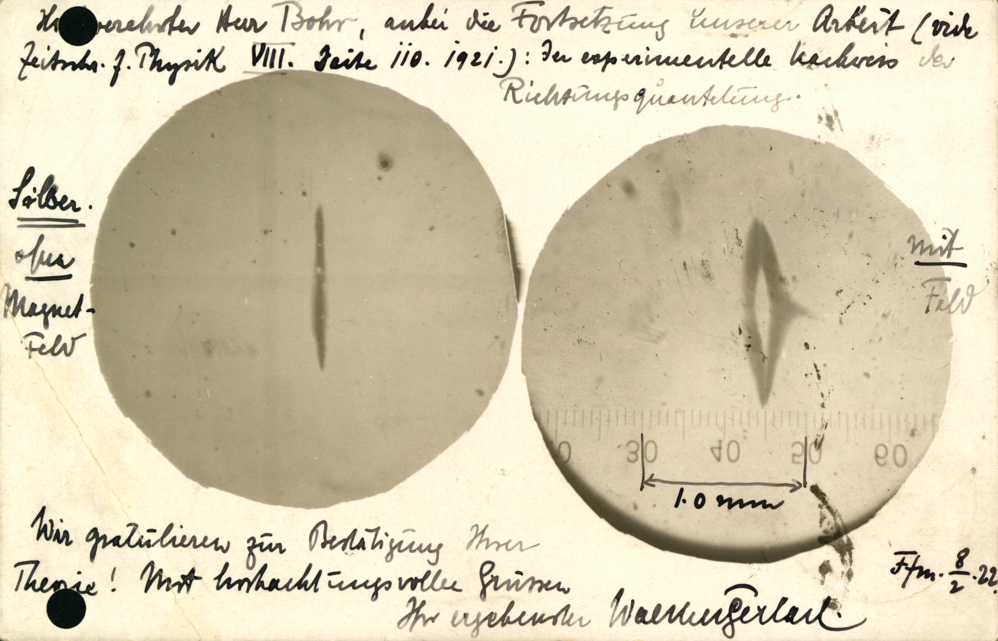
Historical note: A postcard to Bohr

The excitement of the discovery is nicely captured in a postcard Walter Gerlach sent to Niels Bohr on February 8, 1922. On the front was a microphotograph showing the silver-beam deposit without and with a magnetic field. The message reads (in translation):

“Dear Professor Bohr, enclosed is the continuation of our work (see Zeitschrift für Physik VIII, p. 110, 1921): the experimental proof of space quantization…. Silver without magnetic field … with field… Congratulations on the confirmation of your theory. Respectfully yours, Walter Gerlach, Frankfurt, 8/2/22.”

This personal note illustrates how strongly the result was seen as confirming the Bohr–Sommerfeld model. Only later was it understood that the observed splitting in fact revealed a new quantum number — the electron’s spin.

Postcard from Walter Gerlach to Niels Bohr (1922), showing a microphotograph of the silver-beam deposit without and with a magnetic field. Courtesy of the Niels Bohr Archive, Copenhagen https://nbarchive.ku.dk/

The Einstein–de Haas experiment

Einstein and de Haas (1915) were motivated by the idea of ring currents — circulating electrons in atomic orbits — as the microscopic origin of magnetization. Their experiment showed directly that reversing the magnetization of a ferromagnetic sample induces mechanical rotation of the whole body, thus establishing the deep connection between magnetic moments and angular momentum.

However, when they compared the proportionality, they encountered a puzzle: the magnetic moment per unit angular momentum came out to be about twice the classical value expected from orbital currents. This discrepancy was a mystery at the time. In their language, it was often expressed as a “gyromagnetic ratio” differing by a factor of two from theoretical expectations.

It was only later, with the recognition that the electron carries an intrinsic spin with \(g \approx 2\), that this factor found its natural explanation. In other words, the Einstein–de Haas effect had already measured the electron’s \(g\)-factor without knowing that spin existed.

Synthesis

From today’s perspective, both experiments provided indirect evidence for electron spin long before the concept was articulated. But historically, they were interpreted through the lens of orbital angular momentum:

• Stern–Gerlach: seen as proof of spatial quantization of orbital angular momentum projections, though the peculiar “two-spot” pattern foreshadowed something deeper.
  
• Einstein–de Haas: seen as proof that magnetism stems from angular momentum, though the anomalous factor of two hinted at a hidden degree of freedom.

Only with Pauli’s exclusion principle (1925) and the proposal of electron spin by Uhlenbeck and Goudsmit (1925) were these puzzles fully understood. The reinterpretation of these classic experiments thus marks a turning point in atomic physics — from the orbital models of Bohr–Sommerfeld to the modern framework of quantum mechanics with spin.

---

2. The Electron Spin

Electrons possess an intrinsic angular momentum called spin (\(\hat{\vec{S}}\)). Unlike orbital angular momentum, spin has no classical analog: it is a purely quantum property that must be described algebraically.

The spin operator satisfies the same eigenvalue equations as orbital angular momentum:

\[ \hat{\vec{S}}^2 |s,m_s\rangle = \hbar^2 s(s+1)\,|s,m_s\rangle, \qquad \hat{S}_z |s,m_s\rangle = \hbar m_s\,|s,m_s\rangle. \]

In addition, the spin components obey the same commutation relations as the orbital angular momentum operators:

\[ [\hat{S}_i, \hat{S}_j] = i\hbar\,\varepsilon_{ijk}\,\hat{S}_k, \]

with \(\varepsilon_{ijk}\) the Levi-Civita symbol.

For a single electron, the spin quantum number \(s\) and the magnetic spin quantum number \(m_s\) take the values:

\[ \begin{align} s &= \tfrac{1}{2}\\ m_s &= \pm \tfrac{1}{2} \end{align} \]

2.1 Notation

It is conventional to introduce the shorthand:

• Spin-up: \(|\tfrac{1}{2}, +\tfrac{1}{2}\rangle \equiv |\uparrow\rangle \equiv \begin{pmatrix}1 \\ 0\end{pmatrix}\)
• Spin-down: \(|\tfrac{1}{2}, -\tfrac{1}{2}\rangle \equiv |\downarrow\rangle \equiv \begin{pmatrix}0 \\ 1\end{pmatrix}\)

Unlike orbital states, there is no spatial wavefunction representation for spin alone. Electron spin is a purely quantum property and does not correspond, as orbital angular momentum does, to the rotation of an object in space. Therefore, there is no coordinate-space representation of the spin operator (such as a differential operator) and no spatial wavefunction for spin. Instead, spin states are always described algebraically by two-component spinors.

2.2 Spin Operators

To satisfy the eigenvalue and commutation relations, the spin operators are represented using the Pauli matrices, which provide a concrete \(2\times 2\) matrix representation of spin-\(\tfrac{1}{2}\) systems. Unlike orbital angular momentum, which is represented by differential operators acting on spatial wavefunctions, spin has no spatial representation and is instead described purely through this matrix formalism.

\[ \hat{S}_x = \frac{\hbar}{2}\,\sigma_x, \qquad \hat{S}_y = \frac{\hbar}{2}\,\sigma_y, \qquad \hat{S}_z = \frac{\hbar}{2}\,\sigma_z, \]

where

\[ \sigma_x = \begin{pmatrix}0 & 1 \\ 1 & 0\end{pmatrix}, \quad \sigma_y = \begin{pmatrix}0 & -i \\ i & 0\end{pmatrix}, \quad \sigma_z = \begin{pmatrix}1 & 0 \\ 0 & -1\end{pmatrix}. \]

NoteProof

1. Commutator relations

We want to show that \[ [\hat{S}_i, \hat{S}_j] = i \hbar \, \varepsilon_{ijk} \hat{S}_k \] for \(i,j,k = x,y,z\).

Step 1: Write \(\hat{S}_i = \frac{\hbar}{2}\sigma_i\), then \[ [\hat{S}_i, \hat{S}_j] = \frac{\hbar^2}{4} [\sigma_i, \sigma_j]. \]

Step 2: Recall the Pauli matrix commutators: \[ [\sigma_x, \sigma_y] = 2i \sigma_z, \quad [\sigma_y, \sigma_z] = 2i \sigma_x, \quad [\sigma_z, \sigma_x] = 2i \sigma_y. \]

Step 2: Compute the commutators of the Pauli matrices.

• Example: compute \([\sigma_x, \sigma_y] = \sigma_x \sigma_y - \sigma_y \sigma_x\): \[ \sigma_x \sigma_y = \begin{pmatrix}0 & 1 \\ 1 & 0\end{pmatrix} \begin{pmatrix}0 & -i \\ i & 0\end{pmatrix} = \begin{pmatrix} i & 0 \\ 0 & -i \end{pmatrix} = i \sigma_z, \]

\[ \sigma_y \sigma_x = \begin{pmatrix}0 & -i \\ i & 0\end{pmatrix} \begin{pmatrix}0 & 1 \\ 1 & 0\end{pmatrix} = \begin{pmatrix}-i & 0 \\ 0 & i \end{pmatrix} = -i \sigma_z. \]

• Therefore, \[ [\sigma_x, \sigma_y] = \sigma_x \sigma_y - \sigma_y \sigma_x = i\sigma_z - (-i\sigma_z) = 2i \sigma_z. \]

• Similarly, \[ [\sigma_y, \sigma_z] = 2i \sigma_x, \quad [\sigma_z, \sigma_x] = 2i \sigma_y. \]

This shows explicitly how the commutators arise directly from the matrix multiplication.

Step 3: Multiply by \(\frac{\hbar^2}{4}\): \[ [\hat{S}_x, \hat{S}_y] = \frac{\hbar^2}{4} \cdot 2i \sigma_z = i\hbar \hat{S}_z, \] and similarly for the other pairs.

---

2. Squared spin operator \(\hat{\mathbf{S}}^2\)

\(\hat{\mathbf{S}}^2 = \hat{S}_x^2 + \hat{S}_y^2 + \hat{S}_z^2\).

Step 1: Substitute the Pauli matrices: \[ \hat{S}_x^2 = \left(\frac{\hbar}{2}\right)^2 \sigma_x^2, \quad \hat{S}_y^2 = \left(\frac{\hbar}{2}\right)^2 \sigma_y^2, \quad \hat{S}_z^2 = \left(\frac{\hbar}{2}\right)^2 \sigma_z^2. \]

Step 2: Use \(\sigma_i^2 = I_2\) for all Pauli matrices: \[ \hat{\mathbf{S}}^2 = \frac{\hbar^2}{4} (I_2 + I_2 + I_2) = \frac{3}{4} \hbar^2 I_2. \]

Step 3: Action on spinors: \[ \hat{\mathbf{S}}^2 |\uparrow\rangle = \frac{3}{4}\hbar^2 |\uparrow\rangle, \quad \hat{\mathbf{S}}^2 |\downarrow\rangle = \frac{3}{4}\hbar^2 |\downarrow\rangle \]

\(\Rightarrow \hat{\mathbf{S}}^2 |s,m_s\rangle = \hbar^2 s(s+1)\,|s,m_s\rangle.\)

---

3. z-component \(\hat{S}_z\)

\(\hat{S}_z = \frac{\hbar}{2} \sigma_z = \frac{\hbar}{2} \begin{pmatrix}1 & 0 \\ 0 & -1\end{pmatrix}\).

Step 1: Apply to spin-up: \[ \hat{S}_z |\uparrow\rangle = \frac{\hbar}{2} \begin{pmatrix}1 & 0 \\ 0 & -1\end{pmatrix} \begin{pmatrix}1 \\ 0\end{pmatrix} = \frac{\hbar}{2} \begin{pmatrix}1 \\ 0\end{pmatrix} = \frac{\hbar}{2} |\uparrow\rangle \]

Step 2: Apply to spin-down: \[ \hat{S}_z |\downarrow\rangle = \frac{\hbar}{2} \begin{pmatrix}1 & 0 \\ 0 & -1\end{pmatrix} \begin{pmatrix}0 \\ 1\end{pmatrix} = -\frac{\hbar}{2} |\downarrow\rangle \]

\(\Rightarrow \hat{S}_z |s,m_s\rangle = \hbar m\,|s,m_s\rangle.\)

These steps explicitly show the commutation relations and eigenvalues for spin-\(\frac{1}{2}\) operators.

2.3 Spin in Hydrogen States

When spin is included, the state of the electron in the hydrogen atom must be specified not only by the spatial quantum numbers \((n, \ell, m_\ell)\) but also by the spin quantum numbers \((s, m_s)\).

A complete basis state can thus be written as

\[ |n, \ell, m_\ell, s, m_s\rangle, \]

where:
- \(n\) is the principal quantum number,
- \(\ell\) is the orbital angular momentum quantum number,
- \(m_\ell\) is the magnetic quantum number of orbital angular momentum,
- \(s = \tfrac{1}{2}\) for an electron,
- \(m_s = \pm \tfrac{1}{2}\) is the spin projection.

This notation emphasizes that the electron’s state is a tensor product of its orbital part \(|n,\ell,m_\ell\rangle\) and its spin part \(|s,m_s\rangle\).

---

3. Magnetic Moments

The angular momentum of an electron is associated with a magnetic moment \(\vec \mu\). There are two contributions:

• Orbital magnetic moment: \[ \vec{\mu}_\ell = g_\ell \, \mu_B \, \vec{L}, \quad \text{with } g_\ell = 1 \]
• Spin magnetic moment: \[ \vec{\mu}_s = g_s \, \mu_B \, \vec{S}, \quad \text{with } g_s \approx 2 \]

Here, \(g\) is the g-factor, and \(\mu_B = \frac{e\hbar}{2m_e}\) is the Bohr magneton.

For orbital angular momentum, \(g_\ell = 1\), which reproduces the classical relation between angular momentum and magnetic moment derived from Larmor theory. That is, a circulating charge creates a magnetic dipole proportional to its angular momentum, in full agreement with classical electrodynamics.

For the electron spin, \(g_s \approx 2\), which cannot be explained classically. This value emerges rigorously from relativistic quantum mechanics via the Dirac equation (not derived here), and it is confirmed experimentally, for example in the Einstein–de Haas experiment (1915). The factor \(g_s \neq 1\) is therefore a pure quantum-relativistic effect, reflecting the intrinsic nature of spin.

---

4. The Fine Structure Interaction

4.1 Spin–Orbit Interaction and the Hamiltonian

Because both orbital and spin angular momenta give rise to magnetic moments, they interact with each other. This interaction contributes an additional spin–orbit term, \(\hat{H}_{\rm SO}\), to the Hamiltonian. Including spin, a convenient operator form of the one-electron Hamiltonian in a central potential \(V(\hat{\vec r})\) is

\[ \hat{H} \;=\; \frac{\hat{\vec p}^{\,2}}{2\mu} \;+\; V(\hat{\vec r}) \;+\; \hat{H}_{\rm SO}, \]

where \(\hat{\mathbf p}\) is the momentum operator, \(\mu\) the (reduced) mass, and \(\hat{H}_{\rm SO}\) denotes the spin–orbit interaction, which arises due to the interaction of the magnetic moments and is

\[ \hat{H}_{\rm SO} \propto \hat{\vec{\mu}}_\ell \cdot \hat{\vec{\mu}}_s \propto \hat{\vec{L}} \cdot \hat{\vec{S}} = \hat{L}_x\hat{S}_x + \hat{L}_y\hat{S}_y + \hat{L}_z\hat{S}_z. \]

Note

For a central potential \(V(r)\) the standard spin–orbit term (obtained from the Dirac equation or from semi-classical Thomas-corrected arguments) can be written as

\[ \hat{H}_{\rm SO} \;=\; \frac{1}{2m^2 c^2}\,\frac{1}{r}\frac{dV}{dr}\;\hat{\vec L}\!\cdot\!\hat{\vec S}, \]

where \(r=|\hat{\vec r}|\), \(\hat{\vec L}\) is the orbital angular momentum operator and \(\hat{\mathbf S}\) the spin operator. (For the Coulomb potential \(V(r)=-\dfrac{Ze^2}{4\pi\varepsilon_0 r}\) the radial factor becomes proportional to \(1/r^3\); here we keep the general \(V(r)\) form.)

Because \(\hat{H}_{\rm SO}\) contains \(\hat{\mathbf L}\cdot\hat{\mathbf S}\), the full Hamiltonian no longer commutes with \(\hat{L}_z\) or \(\hat{S}_z\) separately. Formally,

\[ [\hat{H},\hat{L}_z] \;=\; [\hat{H}_{\rm SO},\hat{L}_z] \quad\text{and}\quad [\hat{H},\hat{S}_z] \;=\; [\hat{H}_{\rm SO},\hat{S}_z]. \]

NoteProof

To see that these commutators are nonzero, compute (componentwise) the commutator of \(\hat{\mathbf L}\!\cdot\!\hat{\mathbf S}\) with \(\hat{L}_z\):

\[ \begin{aligned} \big[\hat{\mathbf L}\!\cdot\!\hat{\mathbf S},\,\hat{L}_z\big] &= \big[L_x S_x + L_y S_y + L_z S_z,\; L_z\big] \\ &= [L_x,L_z]\,S_x + [L_y,L_z]\,S_y + [L_z,L_z]\,S_z \\ &= -i\hbar\,L_y S_x - i\hbar\,L_x S_y \\ &= -i\hbar\,(L_y S_x + L_x S_y), \end{aligned} \]

which is generally nonzero (it vanishes only for special states). Hence

\[ [\hat{H},\hat{L}_z] \;=\; \text{(nonzero)} \quad\Rightarrow\quad \hat{L}_z \text{ is not conserved when } \hat{H}_{\rm SO}\neq 0. \]

Similarly, using \([S_i,S_j]=i\hbar\varepsilon_{ijk}S_k\),

\[ \begin{aligned} \big[\hat{\mathbf L}\!\cdot\!\hat{\mathbf S},\,\hat{S}_z\big] &= L_x\,[S_x,S_z] + L_y\,[S_y,S_z] + L_z\,[S_z,S_z] \\ &= -i\hbar\,L_x S_y + i\hbar\,L_y S_x \\ &= i\hbar\,(L_y S_x - L_x S_y), \end{aligned} \]

so

\[ [\hat{H},\hat{S}_z] \;=\; \text{(nonzero)} \quad\Rightarrow\quad \hat{S}_z \text{ is not conserved when } \hat{H}_{\rm SO}\neq 0. \]

Because \(\hat{L}_z\) and \(\hat{S}_z\) do not commute with the Hamiltonian containing spin–orbit coupling, the state \(|n, \ell, m_\ell, s, m_s\rangle\) is not an eigenstate of the Hamiltonian anymore and the quantum numbers \(m_\ell\) and \(m_s\) are no longer conserved.

4.2 The Total Electron Angular Momentum

The solution is to introduce the total electron angular momentum, \(\hat{\vec{J}} = \hat{\vec{L}} + \hat{\vec{S}}\). We can express the interaction term using the total angular momentum:

\[ \hat{\vec{J}}^2 = \hat{\vec{L}}^2 + \hat{\vec{S}}^2 + 2\,\hat{\vec{L}}\cdot\hat{\vec{S}} \quad\Longrightarrow\quad \hat{\vec{L}}\cdot\hat{\vec{S}} = \tfrac{1}{2}\big(\hat{\vec{J}}^2 - \hat{\vec{L}}^2 - \hat{\vec{S}}^2\big). \]

The operators \(\hat{J}^2\) and \(\hat{J}_z\) commute with the Hamiltonian, so the quantum numbers \(j\) and \(m_j\) are now conserved. Their eigenvalues follow the standard angular momentum relations:

\[ \begin{align} \hat{\vec{J}}^2|j,m_j\rangle &= \hbar^2 j(j+1)|j,m_j\rangle\\ \hat{J}_z|j,m_j\rangle &= \hbar m_j|j,m_j\rangle \end{align} \]

The possible values for \(j\) are given by the Clebsch-Gordan series:

\[|\ell-s| \le j \le \ell+s.\]

The new complete set of quantum numbers for the hydrogen atom, when spin is included, is

\[ |n,\ell,s,j,m_j\rangle. \]

These states are eigenstates of the Hamiltonian, and therefore provide the most convenient description of the system. The eigenvalue relation of the spin-orbit operator follows

\[ \begin{align} \hat{\vec{L}}\cdot\hat{\vec{S}} |n,\ell,s,j,m_j\rangle = \tfrac{1}{2}\big(\hat{\vec{J}}^2 - \hat{\vec{L}}^2 - \hat{\vec{S}}^2\big) |n,\ell,s,j,m_j\rangle\\ = \frac{\hbar^2}{2}(j(j+1)-\ell(\ell+1)-s(s+1))|n,\ell,s,j,m_j\rangle. \end{align} \]

Illustration of L–S coupling. Total angular momentum J is green, orbital L is blue, and spin S is red (LS_coupling_(corrected) by AnotherFlake under CC BY-SA 4.0)

The new eigenstates can also be written as linear combinations of the “old” basis states \(|n,\ell,m_\ell,s,m_s\rangle\), where the orbital and spin angular momenta were treated separately.

To make this connection, we insert the identity operator expressed in the \(\{|n,\ell,m_\ell,s,m_s\rangle\}\) basis:

\[ |n,\ell,s,j,m_j\rangle = \sum_{m_\ell,m_s} |n,\ell,m_\ell,s,m_s\rangle \langle n,\ell,m_\ell,s,m_s \,|\, n,\ell,s,j,m_j\rangle. \]

The overlap coefficients
\[\langle n,\ell,m_\ell,s,m_s \,|\, n,\ell,s,j,m_j\rangle\]
are precisely the Clebsch–Gordan coefficients, which describe how to combine orbital and spin angular momenta into total angular momentum.

Thus, the new basis states are superpositions of the old \(|m_\ell, m_s\rangle\) states, weighted by these coefficients.

NoteNote: The Identity Operator in a Complete Basis

In quantum mechanics, a set of states \(\{|a_i\rangle\}\) is called a complete orthonormal basis if:

1. \(\langle a_i | a_j \rangle = \delta_{ij}\) (orthonormality)
   
2. The set spans the whole Hilbert space (completeness).

For such a basis, the identity operator can be written as:

\[ \hat{I} = \sum_i |a_i\rangle \langle a_i|. \]

This operator acts like the “do nothing” operator, since for any state \(|\psi\rangle\):

\[ \hat{I}|\psi\rangle = \sum_i |a_i\rangle \langle a_i|\psi\rangle = |\psi\rangle. \]

In our case, the “old” states \(\{|n,\ell,m_\ell,s,m_s\rangle\}\) form a complete basis, so we may freely insert

\[ \hat{I} = \sum_{m_\ell,m_s} |n,\ell,m_\ell,s,m_s\rangle \langle n,\ell,m_\ell,s,m_s|. \]

This is how the new coupled states \(|n,\ell,s,j,m_j\rangle\) can be expressed as superpositions of the old ones.

4.3 Eigenenergies

If we include the spin–orbit interaction in the Hamiltonian

\[ \hat{H} \;=\; \frac{\hat{\vec p}^{\,2}}{2\mu} \;+\; V(\hat{\vec r}) \;+\; \hat{H}_{\rm SO}, \]

then the energy levels can no longer be labeled only by \(n\).
Instead, they split according to the total angular momentum quantum number \(j\) and the orbital angular momentum quantum number \(\ell\), so the eigenenergies depend on the set \((n, \ell, j)\).

However, this approach is incomplete. A fully consistent calculation of the fine structure requires additional relativistic corrections, which we do not discuss here in detail:

• the Darwin term, arising from the “zitterbewegung” of the electron,
  
• and the Thomas precession correction, which modifies the effective strength of the spin–orbit interaction.

When these effects are combined with the spin–orbit coupling, the result is the same fine structure spectrum that is obtained directly from the Dirac equation.

In the Dirac theory, the energy levels of hydrogen-like atoms (including the rest energy of the electron) are given by

\[ E_{n,j} \;=\; m c^2 \left[ 1 + \left( \frac{Z \alpha}{n - (j + \tfrac{1}{2}) + \sqrt{(j+\tfrac{1}{2})^2 - (Z\alpha)^2}} \right)^2 \right]^{-\tfrac{1}{2}} , \]

where \(\alpha\) (\(\alpha=\tfrac{1}{137}\)) is the fine-structure constant and \(Z\) is the nuclear charge.

The above energies depend only on \(n\) and \(j\). Thus, while the Schrödinger equation with spin–orbit interaction suggests a dependence on \(\ell\), the full relativistic treatment (or including the missing correction terms) removes this \(\ell\)-dependence.

---

4.4 Fine-Structure Energy Shift

It is often more useful to consider the fine-structure shift rather than the full electron energy given above. This shift can be viewed as a small correction to the non-relativistic Bohr energies, which are expressed as:

\[ E_n^{(0)} = - \frac{\mu c^2 (Z\alpha)^2}{2 n^2}, \]

where \(\mu\) is the reduced mass of the electron. To leading order in \((Z\alpha)^2\), the shift due to relativistic effects and spin–orbit interaction becomes

\[ \Delta E_{n,j}^{\rm FS} = E_n^{(0)} \, (Z\alpha)^2 \left( \frac{1}{n} \frac{1}{j + 1/2} - \frac{3}{4 n^2} \right). \]

Thus, the total energy including fine structure is

\[ E_{n,j} \approx E_n^{(0)} + \Delta E_{n,j}^{\rm FS}. \]

Notes:

• The first term in parentheses arises from the spin–orbit interaction.
  
• The second term arises from the relativistic correction to the kinetic energy.
  
• As in the full Dirac theory, the energy now depends on \(n\) and \(j\), but not on \(\ell\) individually, consistent with experiment.

---

5. Term Symbols and Naming Conventions

In atomic and molecular physics (AMO), term symbols are used to describe the electronic states, including the splitting due to the fine structure. The general notation is:

\[{}^{2S+1}L_J\]

• n: The principal quantum number (sometimes included).
• \(2S+1\): The multiplicity.
• L: A letter representing the orbital angular momentum quantum number \(l\).
  • \(l=0 \implies S\)
  • \(l=1 \implies P\)
  • \(l=2 \implies D\)
  • \(l=3 \implies F\)
  • …
• J: The total angular momentum quantum number \(j\).

The splitting of energy levels due to different values of \(j\) is known as fine structure.