2.7 Quantization of the Electromagnetic Field

From classical electrodynamics to photons

Introduction

The quantum harmonic oscillator is more than a model for a particle moving near a stable equilibrium. It also provides the mathematical framework for describing the electromagnetic field quantum mechanically. The central result of this chapter is that each independent normal mode of the free electromagnetic field is equivalent to a harmonic oscillator. Its quantized excitations are photons.

Establishing this connection requires concepts from classical mechanics and electrodynamics that go beyond the usual introductory physics curriculum. These include the Lagrangian and Hamiltonian formulations of mechanics, electromagnetic potentials, gauge transformations, and the energy of electromagnetic fields. A complete and mathematically rigorous treatment would require considerably more background and is beyond the scope of this course.

This chapter therefore aims to strike a balance between theoretical foundations and practical relevance. Rather than developing all the underlying classical theory from first principles, we introduce the essential concepts and use them to motivate the quantization of the electromagnetic field. The emphasis is on understanding the physical principles and the origin of the results that we will use in atomic, molecular, and optical physics.

We begin by examining how charged particles interact with classical electromagnetic potentials, leading to the minimal-coupling Hamiltonian. We then describe the electromagnetic field in terms of independent normal modes and show how their quantization leads to photons, vacuum fluctuations, and different quantum states of light.

These results provide the foundation for the quantum description of light–matter interactions developed later in this course, particularly the treatment of atomic transitions, photon absorption, and spontaneous emission in Chapter 5.

ImportantCore Knowledge — Know

Electromagnetic potentials and minimal coupling

The electromagnetic fields are expressed in terms of the scalar and vector potentials:

\[ \boxed{ \vec E=-\vec\nabla\phi-\frac{\partial\vec A}{\partial t}, \qquad \vec B=\vec\nabla\times\vec A. } \]

For a particle of charge \(q\), the canonical momentum and minimal-coupling Hamiltonian are

\[ \boxed{ \vec p=m\vec v+q\vec A, \qquad H=\frac{(\vec p-q\vec A)^2}{2m}+q\phi. } \]

In the Coulomb gauge, \(\vec\nabla\cdot\vec A=0\), the independent radiation degrees of freedom are transverse.

Quantization of the electromagnetic field

Each independent transverse electromagnetic mode behaves as a harmonic oscillator. Promoting its canonical variables \(q_s\) and \(p_s\) to operators gives

\[ [\hat q_s,\hat p_{s'}]=i\hbar\delta_{ss'}. \]

The quantized electromagnetic-field Hamiltonian can be written as

\[ \boxed{ \hat H_{\mathrm{EM}} =\sum_s\left( \frac{\hat p_s^2}{2} +\frac{\omega_s^2\hat q_s^2}{2} \right) =\sum_s\hbar\omega_s \left(\hat a_s^\dagger\hat a_s+\frac12\right). } \]

The creation and annihilation operators satisfy

\[ [\hat a_s,\hat a_{s'}^\dagger]=\delta_{ss'}, \]

and act on photon-number states according to

\[ \hat a_s|n_s\rangle=\sqrt{n_s}\,|n_s-1\rangle, \qquad \hat a_s^\dagger|n_s\rangle=\sqrt{n_s+1}\,|n_s+1\rangle. \]

Each photon contributes an energy \(\hbar\omega_s\) to its electromagnetic mode.

Quantum states and uncertainty

For a single electromagnetic mode, the field quadratures are

\[ \boxed{ \hat X=\sqrt{\frac{\omega}{2\hbar}}\,\hat q =\frac{\hat a+\hat a^\dagger}{2}, \qquad \hat Y=\frac{\hat p}{\sqrt{2\hbar\omega}} =\frac{\hat a-\hat a^\dagger}{2i}. } \]

with the uncertainty relation

\[ \boxed{\Delta X\,\Delta Y\geq\frac14.} \]

Three important quantum states of light are:

• Fock states \(|n\rangle\): definite photon number, \(\Delta N=0\), and vanishing mean electric field.

• Coherent states \(|\alpha\rangle\): eigenstates of \(\hat a\), with Poissonian photon-number statistics,

  \[ (\Delta N)^2=\langle N\rangle=|\alpha|^2. \]

• Squeezed states: reduced uncertainty in one quadrature at the expense of increased uncertainty in the other.

NoteWorking Knowledge — Understand

Electromagnetic potentials and minimal coupling

• Gauge transformations change the scalar and vector potentials without changing the physical electromagnetic fields.
• Canonical momentum differs from mechanical momentum in the presence of a vector potential. This distinction leads to the minimal-coupling Hamiltonian.
• In Coulomb gauge, the longitudinal electric field describes electrostatic interactions, while the transverse field contains the independent radiation degrees of freedom.

Classical field Hamiltonian

• The electromagnetic field can be decomposed into independent normal modes, each equivalent to a harmonic oscillator.
• The canonical variables \(q_s\) and \(p_s\) describe field modes, not the position and momentum of individual photons.
• The classical field energy becomes a sum of harmonic-oscillator Hamiltonians.

Quantization of the electromagnetic field

• Quantizing the normal modes introduces photon creation and annihilation operators.
• Photons are quantum excitations of electromagnetic modes, characterized by their frequency, spatial structure, and polarization.
• The vacuum state contains no photons but still possesses zero-point energy and nonzero field fluctuations.

Quantum states and uncertainty

• Fock states have definite photon number but no preferred optical phase. Their mean electric field vanishes, although they can still exhibit interference.
• Coherent states most closely resemble classical electromagnetic waves, with an oscillating mean electric field and equal quadrature uncertainties.
• Squeezed states redistribute quantum fluctuations. Amplitude squeezing reduces fluctuations along the mean field amplitude, while phase squeezing reduces fluctuations perpendicular to it.
• Squeezing can improve optical measurement precision by reducing quantum noise in the relevant quadrature, without violating the uncertainty principle.

The detailed derivations of minimal coupling, the normal-mode expansion, and field quantization are included to explain how the quantum description of light emerges from classical electrodynamics. The intermediate algebra and normalization calculations are not intended as material to memorize.

2.7.1. Charged particles and electromagnetic potentials

A particle of mass \(m\) and charge \(q\) moving with velocity \(\vec v=\dot{\vec r}\) in an electromagnetic field experiences the Lorentz force,

\[ m\ddot{\vec r} =q\left[\vec E(\vec r,t)+\dot{\vec r}\times\vec B(\vec r,t)\right]. \]

The electromagnetic fields themselves are governed by Maxwell’s equations. In SI units, these are

\[ \begin{aligned} \vec\nabla\cdot\vec E &= \frac{\rho}{\varepsilon_0}, &\qquad \vec\nabla\cdot\vec B &= 0,\\[6pt] \vec\nabla\times\vec E &= -\frac{\partial\vec B}{\partial t}, &\qquad \vec\nabla\times\vec B &= \mu_0\vec j+\mu_0\varepsilon_0 \frac{\partial\vec E}{\partial t}. \end{aligned} \]

Here, \(\rho(\vec r,t)\) and \(\vec j(\vec r,t)\) denote the electric charge and current densities, respectively.

Rather than working directly with the electric and magnetic fields, it is often convenient to introduce a scalar potential \(\phi(\vec r,t)\) and a vector potential \(\vec A(\vec r,t)\), such that

\[ \boxed{ \vec E=-\vec\nabla\phi-\frac{\partial\vec A}{\partial t}, \qquad \vec B=\vec\nabla\times\vec A. } \]

These expressions automatically satisfy two of Maxwell’s equations: \(\vec\nabla\cdot\vec B=0\) and \(\vec\nabla\times\vec E=-\partial_t\vec B\). The remaining two Maxwell equations determine the potentials in terms of the charge and current distributions.

An important property of this description is that the potentials are not uniquely determined by the electromagnetic fields. Consider an arbitrary, sufficiently smooth scalar function \(\chi(\vec r,t)\) of position and time. We can define new potentials through the gauge transformation

\[ \boxed{ \vec A'=\vec A+\vec\nabla\chi, \qquad \phi'=\phi-\frac{\partial\chi}{\partial t}. } \]

Although the potentials change, the physical electromagnetic fields remain exactly the same. Thus, different choices of \(\chi(\vec r,t)\) correspond to different mathematical descriptions of the same electromagnetic field.

NoteDerivation: Gauge transformations leave the fields unchanged

For the magnetic field, we obtain

\[ \begin{aligned} \vec B' &=\vec\nabla\times\vec A'\\ &=\vec\nabla\times(\vec A+\vec\nabla\chi)\\ &=\vec\nabla\times\vec A +\underbrace{\vec\nabla\times(\vec\nabla\chi)}_{=0}\\ &=\vec B. \end{aligned} \]

For the electric field,

\[ \begin{aligned} \vec E' &=-\vec\nabla\phi'-\frac{\partial\vec A'}{\partial t}\\ &=-\vec\nabla\left(\phi-\frac{\partial\chi}{\partial t}\right) -\frac{\partial}{\partial t} \left(\vec A+\vec\nabla\chi\right)\\ &=-\vec\nabla\phi-\frac{\partial\vec A}{\partial t} +\underbrace{\vec\nabla\frac{\partial\chi}{\partial t} -\frac{\partial}{\partial t}(\vec\nabla\chi)}_{=0}\\ &=\vec E. \end{aligned} \]

Here we used the fact that spatial and temporal derivatives commute for sufficiently smooth functions.

2.7.2. Minimal coupling from the classical Lagrangian

In Newtonian mechanics, the motion of a particle is determined by Newton’s second law, \(\vec F=m\ddot{\vec r}\). An equivalent description is provided by Lagrangian mechanics, which formulates the equations of motion in terms of a single function, the Lagrangian \(L\).

For a particle moving in a conservative potential \(V(\vec r)\), the Lagrangian is simply the difference between kinetic and potential energy,

\[ L=T-V=\frac12m\dot{\vec r}^{\,2}-V(\vec r). \]

More generally, the equations of motion follow from the principle of stationary action: the actual trajectory between two fixed endpoints makes the action

\[ S=\int_{t_i}^{t_f}L\,dt \]

stationary with respect to small variations of the trajectory. This leads to the Euler–Lagrange equations (also called Lagrange’s equations of the second kind),

\[ \boxed{ \frac{d}{dt}\frac{\partial L}{\partial\dot x_i} -\frac{\partial L}{\partial x_i}=0. } \]

For \(L=T-V\), these equations reproduce Newton’s second law, \(m\ddot{\vec r}=-\vec\nabla V\). Thus, Lagrangian mechanics does not introduce different physics; it provides another way of describing the same motion.

2.7.2.1 The Lagrangian of a charged particle

For a charged particle in an electromagnetic field, the situation is slightly more complicated. The magnetic part of the Lorentz force, \(q\vec v\times\vec B\), depends on the particle’s velocity and therefore cannot be obtained from an ordinary position-dependent potential energy \(V(\vec r)\).

Instead, the electromagnetic interaction requires a velocity-dependent term in the Lagrangian. For a particle of mass \(m\) and charge \(q\) moving in prescribed electromagnetic potentials \(\phi(\vec r,t)\) and \(\vec A(\vec r,t)\), we use

\[ \boxed{ L=\frac12m\dot{\vec r}^{\,2} +q\dot{\vec r}\cdot\vec A(\vec r,t) -q\phi(\vec r,t). } \]

The first term is the kinetic energy. The term \(-q\phi\) describes the interaction with the scalar potential, while \(q\dot{\vec r}\cdot\vec A\) accounts for the velocity-dependent electromagnetic interaction.

Why is this the correct Lagrangian? We can establish its consistency with classical electrodynamics by checking two essential properties:

1. Lorentz force: The Euler–Lagrange equations must reproduce the familiar equation of motion \(m\ddot{\vec r}=q(\vec E+\vec v\times\vec B)\).

2. Gauge invariance: Changing the electromagnetic potentials by a gauge transformation must not change the particle’s physical motion.

We verify the first property below. The second will be demonstrated after introducing the canonical momentum and Hamiltonian.

NoteDerivation: recover the Lorentz force, component by component

For a Cartesian coordinate \(x_i\), the Euler–Lagrange equation is

\[ \frac{d}{dt}\frac{\partial L}{\partial\dot x_i} -\frac{\partial L}{\partial x_i}=0. \]

First,

\[ \frac{\partial L}{\partial\dot x_i}=m\dot x_i+qA_i, \]

and therefore, using the chain rule along the trajectory,

\[ \frac{d}{dt}\frac{\partial L}{\partial\dot x_i} =m\ddot x_i+q\partial_t A_i +q\sum_j\dot x_j\partial_j A_i. \]

On the other hand,

\[ \frac{\partial L}{\partial x_i} =q\sum_j\dot x_j\partial_i A_j-q\partial_i\phi. \]

Combining the two expressions gives

\[ m\ddot x_i=q(-\partial_i\phi-\partial_t A_i) +q\sum_j\dot x_j(\partial_i A_j-\partial_j A_i). \]

The first parentheses equal \(E_i\). The vector identity

\[ (\mathbf v\times(\boldsymbol\nabla\times\mathbf A))_i =\sum_jv_j(\partial_iA_j-\partial_jA_i) \]

identifies the second term as \((\mathbf v\times\mathbf B)_i\). Thus

\[ m\ddot{\mathbf r}=q(\mathbf E+\mathbf v\times\mathbf B). \]

2.7.2.2 From Lagrangian to Hamiltonian mechanics

The Lagrangian formulation describes the motion of a particle in terms of its position \(\vec r\) and velocity \(\dot{\vec r}\). There is, however, another equivalent formulation of classical mechanics that is particularly useful for our purposes: Hamiltonian mechanics.

Instead of working with positions and velocities, Hamiltonian mechanics uses positions and momenta as its fundamental variables. Together, these define the phase space of a system, which combines position and momentum space. A point in phase space specifies the instantaneous state of a classical system.

To make this change of variables, we first need to define the momentum associated with each coordinate. In Lagrangian mechanics, this is done through

\[ \boxed{ p_i=\frac{\partial L}{\partial\dot x_i}. } \]

This quantity is called the canonical momentum, or the momentum conjugate to the coordinate \(x_i\). The term conjugate indicates that \(x_i\) and \(p_i\) form a corresponding pair of phase-space coordinates.

For the familiar Lagrangian \(L=T-V\), where the potential energy does not depend on velocity, we find

\[ p_i=\frac{\partial}{\partial\dot x_i} \left(\frac12m\dot{\vec r}^{\,2}-V\right) =m\dot x_i. \]

Thus, in this case, canonical momentum is identical to the familiar mechanical momentum \(m\dot{\vec r}\).

For a charged particle in an electromagnetic field, however, the Lagrangian contains an additional velocity-dependent term, \(q\dot{\vec r}\cdot\vec A\). Consequently,

\[ \boxed{ \vec p=\frac{\partial L}{\partial\dot{\vec r}} =m\dot{\vec r}+q\vec A. } \]

The canonical momentum therefore differs from the mechanical momentum:

\[ \boxed{ \underbrace{m\dot{\vec r}}_{\text{mechanical momentum}} = \underbrace{\vec p}_{\text{canonical momentum}} -q\vec A. } \]

This distinction is important because the canonical momentum is the variable used in Hamiltonian mechanics and, subsequently, in the canonical formulation of quantum mechanics.

2.7.2.3 The Hamiltonian and minimal coupling

Having introduced positions and canonical momenta as our new variables, we now need a function that describes the dynamics in terms of these variables.

In Lagrangian mechanics, this role is played by the Lagrangian \(L(\vec r,\dot{\vec r},t)\). In Hamiltonian mechanics, it is played by the Hamiltonian \(H(\vec r,\vec p,t)\).

The two functions are related by a mathematical transformation known as the Legendre transformation:

\[ \boxed{ H=\vec p\cdot\dot{\vec r}-L. } \]

This transformation replaces the dependence on velocity by a dependence on canonical momentum. In particular, the velocities on the right-hand side must be expressed in terms of \(\vec r\) and \(\vec p\).

The Hamiltonian determines the time evolution of the phase-space coordinates through Hamilton’s equations,

\[ \boxed{ \dot x_i=\frac{\partial H}{\partial p_i}, \qquad \dot p_i=-\frac{\partial H}{\partial x_i}. } \]

These equations are equivalent to the Euler–Lagrange equations and therefore to Newton’s equations of motion. They simply express the same physics in terms of positions and momenta rather than positions and velocities.

For a particle with the familiar Lagrangian \(L=T-V\), the Legendre transformation gives

\[ H=\frac{\vec p^{\,2}}{2m}+V(\vec r), \]

which is just the total mechanical energy \(T+V\). This is the Hamiltonian already familiar from elementary quantum mechanics.

We now apply the same procedure to a charged particle in an electromagnetic field. For our electromagnetic Lagrangian, we substitute \(\vec p=m\dot{\vec r}+q\vec A\) and obtain

\[ \begin{aligned} H &=(m\dot{\vec r}+q\vec A)\cdot\dot{\vec r} -\left( \frac12m\dot{\vec r}^{\,2} +q\dot{\vec r}\cdot\vec A-q\phi \right)\\ &=\frac12m\dot{\vec r}^{\,2}+q\phi. \end{aligned} \]

This expression has a familiar form: the kinetic energy plus the electric potential energy. The magnetic field does not contribute a separate potential-energy term.

However, the Hamiltonian must be expressed in terms of the canonical momentum \(\vec p\), rather than the velocity. Using

\[ \dot{\vec r}=\frac{\vec p-q\vec A}{m}, \]

we obtain

\[ \boxed{ H(\vec r,\vec p,t) =\frac{[\vec p-q\vec A(\vec r,t)]^2}{2m} +q\phi(\vec r,t). } \]

This is the minimal-coupling Hamiltonian.

Compared with the Hamiltonian of a free particle, \(H_0=\vec p^{\,2}/(2m)\), the electromagnetic interaction enters through the replacement

\[ \boxed{ \vec p\longrightarrow\vec p-q\vec A, } \]

together with the scalar-potential term \(q\phi\).

The replacement is not an arbitrary prescription. It follows directly from the distinction between canonical and mechanical momentum.

NoteWhy gauge transformations do not change the particle’s motion

Under a gauge transformation,

\[ \vec A'=\vec A+\vec\nabla\chi, \qquad \phi'=\phi-\frac{\partial\chi}{\partial t}, \]

the Lagrangian changes by

\[ \begin{aligned} L'-L &=q\dot{\vec r}\cdot\vec\nabla\chi +q\frac{\partial\chi}{\partial t}\\ &=q\frac{d}{dt}\chi(\vec r(t),t). \end{aligned} \]

The last step uses the chain rule. Notice the distinction between partial and total derivatives:

• The partial derivative \(\partial\chi/\partial t\) describes how \(\chi(\vec r,t)\) changes with time at a fixed position.
• The total derivative \(d\chi/dt\) describes how \(\chi\) changes as we follow the moving particle along its trajectory \(\vec r(t)\).

Since \(\chi\) depends on both position and time,

\[ \boxed{ \frac{d}{dt}\chi(\vec r(t),t) = \underbrace{\dot{\vec r}\cdot\vec\nabla\chi}_{ \text{change due to motion}} + \underbrace{\frac{\partial\chi}{\partial t}}_{ \text{change at fixed position}}. } \]

Thus, the Lagrangian changes by a total time derivative. When we integrate over time to obtain the action, this gives

\[ S'=S+q[\chi(\vec r_f,t_f)-\chi(\vec r_i,t_i)]. \]

Why does this not affect the motion?

Recall that the principle of stationary action compares possible trajectories connecting the same initial and final positions at fixed times.

The additional term depends only on these endpoints, not on the path taken between them. Consequently, every possible trajectory acquires exactly the same additional contribution to its action.

Adding the same constant to the action of every trajectory cannot change which trajectory makes the action stationary.

Therefore, the equations of motion remain unchanged. This establishes the gauge invariance of the particle dynamics, our second consistency requirement.

2.7.2.4 Minimal coupling in quantum mechanics

We can now make the connection to quantum mechanics.

In the position representation, the canonical momentum is represented by the differential operator

\[ \hat{\vec p}=-i\hbar\vec\nabla. \]

Replacing the classical canonical momentum in the minimal-coupling Hamiltonian by this operator gives

\[ \boxed{ \hat H= \frac{1}{2m} \left[-i\hbar\vec\nabla-q\vec A(\vec r,t)\right]^2 +q\phi(\vec r,t). } \]

The corresponding mechanical-momentum operator is

\[ \hat{\vec p}_{\mathrm{mech}} =\hat{\vec p}-q\vec A. \]

An important detail is that \(\hat{\vec p}\) is a differential operator. If \(\vec A\) depends on position, the two generally do not commute. The square in the Hamiltonian therefore represents the complete operator product, including derivatives acting on the vector potential.

NoteProof: Gauge invariance of the Schrödinger equation

Statement. Consider a wavefunction \(\psi(\vec r,t)\) that satisfies the Schrödinger equation

\[ i\hbar\frac{\partial\psi}{\partial t}=\hat H\psi, \]

with the minimal-coupling Hamiltonian

\[ \hat H=\frac{1}{2m}(-i\hbar\vec\nabla-q\vec A)^2+q\phi. \]

We want to demonstrate that a gauge transformation of the electromagnetic potentials,

\[ \vec A'=\vec A+\vec\nabla\chi, \qquad \phi'=\phi-\frac{\partial\chi}{\partial t}, \]

does not change the physical predictions of quantum mechanics.

More precisely, we will show that if \(\psi\) solves the original Schrödinger equation, then the phase-transformed wavefunction

\[ \boxed{ \psi'(\vec r,t)=e^{iq\chi(\vec r,t)/\hbar}\psi(\vec r,t) } \]

solves the Schrödinger equation with the transformed Hamiltonian \(\hat H'\).

Proof. We begin with the momentum-dependent part of the Hamiltonian. In the new gauge, the mechanical-momentum operator is

\[ \hat{\vec p}_{\mathrm{mech}}' =-i\hbar\vec\nabla-q\vec A'. \]

When this operator acts on the transformed wavefunction, the gradient acts on both the exponential phase factor and the original wavefunction. Using the product rule,

\[ \begin{aligned} &\left[-i\hbar\vec\nabla-q\left(\vec A+\vec\nabla\chi\right)\right] \left(e^{iq\chi/\hbar}\psi\right)\\ &\quad= -i\hbar\vec\nabla\left(e^{iq\chi/\hbar}\psi\right) -q\left(\vec A+\vec\nabla\chi\right)e^{iq\chi/\hbar}\psi\\ &\quad= e^{iq\chi/\hbar} \left[ -i\hbar\vec\nabla\psi +q(\vec\nabla\chi)\psi -q\vec A\psi -q(\vec\nabla\chi)\psi \right]\\ &\quad= e^{iq\chi/\hbar} \left(-i\hbar\vec\nabla-q\vec A\right)\psi. \end{aligned} \]

Note: The gradient \(\vec\nabla\chi\) acts only on the gauge function \(\chi\) and is therefore an ordinary vector-valued function. In contrast, the standalone gradient operator \(\vec\nabla\) acts on the entire product \(e^{iq\chi/\hbar}\psi\), requiring the product rule. The two resulting terms involving \(\vec\nabla\chi\) cancel exactly.

Applying the same relation once more shows that the entire kinetic-energy operator transforms in the same way:

\[ \frac{1}{2m}(-i\hbar\vec\nabla-q\vec A')^2\psi' = e^{iq\chi/\hbar} \frac{1}{2m}(-i\hbar\vec\nabla-q\vec A)^2\psi. \]

We must also account for the scalar potential. Since \(\phi'=\phi-\partial_t\chi\), the transformed Hamiltonian acting on \(\psi'\) gives

\[ \boxed{ \hat H'\psi' =e^{iq\chi/\hbar} \left(\hat H\psi-q\frac{\partial\chi}{\partial t}\psi\right). } \]

Now consider the time derivative on the left-hand side of the Schrödinger equation. Because the phase factor also depends on time, the product rule gives

\[ i\hbar\frac{\partial\psi'}{\partial t} =e^{iq\chi/\hbar} \left(i\hbar\frac{\partial\psi}{\partial t} -q\frac{\partial\chi}{\partial t}\psi\right). \]

But the original wavefunction satisfies \(i\hbar\partial_t\psi=\hat H\psi\). Substituting this into the last expression, we obtain

\[ i\hbar\frac{\partial\psi'}{\partial t} =e^{iq\chi/\hbar} \left(\hat H\psi-q\frac{\partial\chi}{\partial t}\psi\right). \]

This is exactly the expression we obtained for \(\hat H'\psi'\). Therefore,

\[ \boxed{ i\hbar\frac{\partial\psi'}{\partial t}=\hat H'\psi'. } \]

Conclusion. The Schrödinger equation retains its form under a gauge transformation, provided the wavefunction acquires the corresponding position- and time-dependent phase factor.

Since this factor has unit magnitude, the probability density is unchanged:

\[ |\psi'(\vec r,t)|^2=|\psi(\vec r,t)|^2. \]

Other physical observables are likewise gauge independent when their operators are transformed consistently. The wavefunction and electromagnetic potentials may change, but they still describe the same physical system.

At this point, the electromagnetic potentials \(\vec A\) and \(\phi\) are still prescribed classical functions. In the following sections, we will describe the electromagnetic field itself as a dynamical system and ultimately quantize its independent degrees of freedom.

2.7.3. Which parts of the electromagnetic field are independent?

In the previous section, we treated the electromagnetic potentials as prescribed classical functions. Our next goal is to describe the electromagnetic field itself as a dynamical system, and eventually to quantize it.

To do so, we must first identify its independent degrees of freedom. For a particle, we can use its position and canonical momentum as dynamical variables. But what are the corresponding variables for an electromagnetic field?

At first glance, we might consider the three components of the electric field \(\vec E\) and the three components of the magnetic field \(\vec B\). However, these six components are not independent: they must satisfy Maxwell’s equations.

In particular, two of Maxwell’s equations,

\[ \vec\nabla\cdot\vec E=\frac{\rho}{\varepsilon_0}, \qquad \vec\nabla\cdot\vec B=0, \]

contain no time derivatives. They impose constraints on the fields at any given instant.

The first equation tells us that the divergence of the electric field is determined by the charge distribution. The second requires the magnetic field to have zero divergence.

The remaining Maxwell equations describe how the electric and magnetic fields evolve in time. Thus, Maxwell’s equations contain both constraints and dynamical equations.

Before quantizing the field, we need to distinguish the parts constrained by the charge distribution from those that can evolve as independent electromagnetic degrees of freedom.

2.7.3.1. The Helmholtz decomposition

A useful mathematical result, known as the Helmholtz decomposition, states that a sufficiently well-behaved vector field can be separated into two parts:

• A longitudinal, or curl-free, component.
• A transverse, or divergence-free, component.

For the electric field, we write

\[ \boxed{ \vec E=\vec E_{\mathrm L}+\vec E_{\mathrm T}, } \]

with

\[ \boxed{ \vec\nabla\times\vec E_{\mathrm L}=0, \qquad \vec\nabla\cdot\vec E_{\mathrm T}=0. } \]

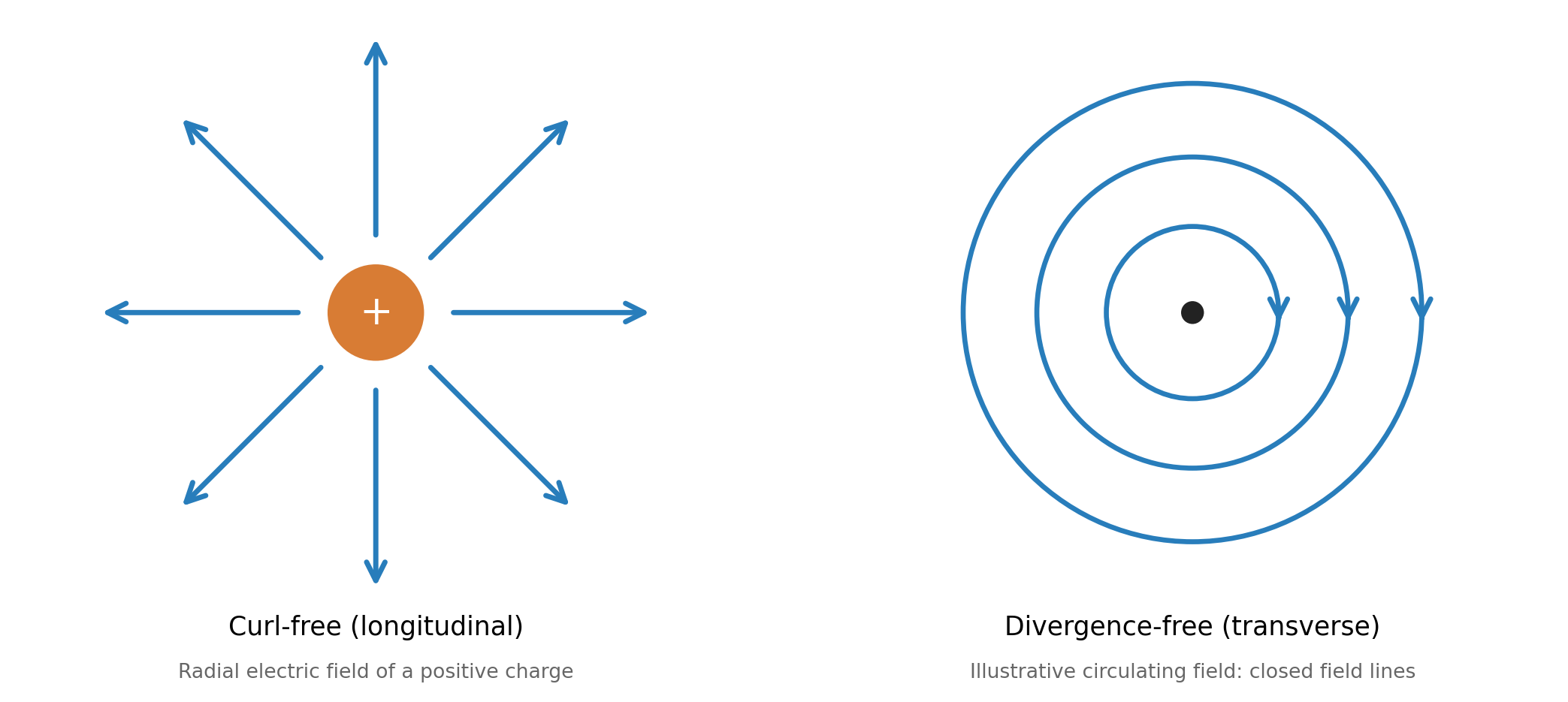
The longitudinal component has no curl, while the transverse component has no divergence.

The terms longitudinal and transverse may seem unusual at this point. For now, they are simply names for these two mathematical properties. Their geometric interpretation will become clearer when we introduce the normal modes of the field.

NoteWhy can a vector field be separated into longitudinal and transverse parts?

The Helmholtz decomposition states that a sufficiently smooth vector field \(\vec F(\vec r)\), with suitable boundary conditions, can be written as

\[ \vec F=\vec F_{\mathrm L}+\vec F_{\mathrm T}, \]

where

\[ \vec\nabla\times\vec F_{\mathrm L}=0, \qquad \vec\nabla\cdot\vec F_{\mathrm T}=0. \]

How can we construct these two components?

We first introduce a scalar function \(\Phi(\vec r)\) satisfying Poisson’s equation,

\[ \nabla^2\Phi=-\vec\nabla\cdot\vec F. \]

We then define the longitudinal component as

\[ \boxed{ \vec F_{\mathrm L}=-\vec\nabla\Phi. } \]

Because the curl of a gradient always vanishes,

\[ \vec\nabla\times\vec F_{\mathrm L} =-\vec\nabla\times(\vec\nabla\Phi)=0. \]

Next, define the remaining part of the field by

\[ \boxed{ \vec F_{\mathrm T}=\vec F-\vec F_{\mathrm L}. } \]

Taking its divergence gives

\[ \begin{aligned} \vec\nabla\cdot\vec F_{\mathrm T} &=\vec\nabla\cdot\vec F -\vec\nabla\cdot\vec F_{\mathrm L}\\ &=\vec\nabla\cdot\vec F+\nabla^2\Phi\\ &=0. \end{aligned} \]

Thus, the first component is curl-free and the second is divergence-free, as required.

For fields that vanish sufficiently rapidly at infinity, Poisson’s equation has the solution

\[ \Phi(\vec r)= \frac{1}{4\pi} \int \frac{\vec\nabla'\cdot\vec F(\vec r')} {|\vec r-\vec r'|} \,d^3r'. \]

This construction establishes the decomposition without assuming that the field describes a wave.

What about the names?

The terms longitudinal and transverse become geometrically transparent when the field is later expanded into spatial Fourier components. For each component, longitudinal means parallel to its spatial wave vector and transverse means perpendicular to it.

That interpretation does not require the field to be an electromagnetic wave; Fourier components can describe arbitrary spatial field distributions.

Why is this decomposition useful?

Consider Gauss’s law. Substituting the decomposition of the electric field gives

\[ \vec\nabla\cdot\vec E_{\mathrm L} +\vec\nabla\cdot\vec E_{\mathrm T} =\frac{\rho}{\varepsilon_0}. \]

By definition, the transverse component has zero divergence. Therefore,

\[ \boxed{ \vec\nabla\cdot\vec E_{\mathrm L} =\frac{\rho}{\varepsilon_0}. } \]

Together with the condition \(\vec\nabla\times\vec E_{\mathrm L}=0\) and suitable boundary conditions, this determines the longitudinal electric field from the charge distribution.

The transverse component, on the other hand, is not determined by Gauss’s law.

We have therefore achieved our first objective: the decomposition separates the electric field constrained by the charges from the part that can possess independent dynamics.

import numpy as np
import matplotlib.pyplot as plt
from matplotlib.patches import Circle, FancyArrowPatch


# ------------------------------------------------------------
# Figure settings
# ------------------------------------------------------------

BLUE = "#287dbb"
ORANGE = "#d87c34"
GRAY = "#666666"

FIELD_WIDTH = 2.6
ARROW_SIZE = 23
CENTER_Y = 0.35

fig, axes = plt.subplots(1, 2, figsize=(11.6, 5.5))

# Both panels use the same coordinate system and have no axes.
for ax in axes:
    ax.set_aspect("equal")
    ax.set_xlim(-2.6, 2.6)
    ax.set_ylim(-2.35, 2.5)
    ax.axis("off")


# ------------------------------------------------------------
# Left panel: longitudinal (curl-free) field
#
# Example: radial electric field of a positive charge.
# The arrows point outward from the charge.
# ------------------------------------------------------------

ax = axes[0]

# Draw the positive charge.
ax.add_patch(
    Circle((0, CENTER_Y), 0.34, color=ORANGE, zorder=3)
)
ax.text(
    0, CENTER_Y, "+",
    color="white", fontsize=20,
    ha="center", va="center", zorder=4
)

# Draw eight equally spaced radial field arrows.
for angle_deg in np.arange(0, 360, 45):
    angle = np.deg2rad(angle_deg)

    start_radius = 0.53
    end_radius = 2.0

    start = (
        start_radius * np.cos(angle),
        CENTER_Y + start_radius * np.sin(angle),
    )
    end = (
        end_radius * np.cos(angle),
        CENTER_Y + end_radius * np.sin(angle),
    )

    ax.add_patch(
        FancyArrowPatch(
            start, end,
            arrowstyle="->",
            mutation_scale=ARROW_SIZE,
            linewidth=FIELD_WIDTH,
            color=BLUE,
        )
    )

ax.text(
    0, -1.97, "Curl-free (longitudinal)",
    ha="center", fontsize=13
)
ax.text(
    0, -2.28, "Radial electric field of a positive charge",
    ha="center", fontsize=10, color=GRAY
)


# ------------------------------------------------------------
# Right panel: transverse (divergence-free) field
#
# Example: a circulating vector field.
# Closed field lines have no beginning or end.
# ------------------------------------------------------------

ax = axes[1]
center = (0, CENTER_Y)

# Mark the center of circulation.
ax.add_patch(
    Circle(center, 0.075, color="#222222", zorder=4)
)

# Draw three circular field lines with clockwise arrows.
for radius in (0.62, 1.12, 1.65):
    ax.add_patch(
        Circle(
            center, radius,
            fill=False,
            edgecolor=BLUE,
            linewidth=2.5,
        )
    )

    # A downward-pointing tangent arrow on the right side
    # indicates clockwise circulation.
    ax.add_patch(
        FancyArrowPatch(
            (radius, CENTER_Y),
            (radius, CENTER_Y - 0.1),
            arrowstyle="->",
            mutation_scale=22,
            linewidth=FIELD_WIDTH,
            color=BLUE,
        )
    )

ax.text(
    0, -1.97, "Divergence-free (transverse)",
    ha="center", fontsize=13
)
ax.text(
    0, -2.28, "Illustrative circulating field: closed field lines",
    ha="center", fontsize=10, color=GRAY
)


# ------------------------------------------------------------
# Final layout
# ------------------------------------------------------------

fig.subplots_adjust(
    left=0.04,
    right=0.96,
    top=0.95,
    bottom=0.10,
    wspace=0.13,
)

plt.show()

Figure 1: Illustration of longitudinal and transverse vector fields. The longitudinal field is curl-free, while the transverse field is divergence-free. The radial and circulating patterns are illustrative examples, not general requirements.

This does not mean that the transverse field is unaffected by charged particles. Currents can generate electromagnetic radiation. The distinction is that the transverse field is not fixed by the instantaneous charge distribution alone.

2.7.3.2. The Coulomb gauge

We now want to express this separation in terms of the electromagnetic potentials introduced earlier.

Recall that

\[ \vec E=-\vec\nabla\phi-\frac{\partial\vec A}{\partial t}, \qquad \vec B=\vec\nabla\times\vec A. \]

Since the electromagnetic potentials are not unique, we can choose a gauge that makes the separation particularly convenient.

We choose the Coulomb gauge, defined by

\[ \boxed{ \vec\nabla\cdot\vec A=0. } \]

In this gauge, the vector potential is divergence-free and therefore purely transverse.

The electric field becomes

\[ \vec E= \underbrace{-\vec\nabla\phi}_{\vec E_{\mathrm L}} \underbrace{-\frac{\partial\vec A}{\partial t}}_{\vec E_{\mathrm T}}. \]

This identification follows directly from the definitions of the two components:

• The gradient of a scalar function is curl-free, so \(-\vec\nabla\phi\) is longitudinal.
• Since \(\vec\nabla\cdot\vec A=0\), its time derivative is also divergence-free, so \(-\partial\vec A/\partial t\) is transverse.

Consequently,

\[ \boxed{ \vec E_{\mathrm L}=-\vec\nabla\phi, \qquad \vec E_{\mathrm T}=-\frac{\partial\vec A}{\partial t}, \qquad \vec B=\vec\nabla\times\vec A. } \]

The Coulomb gauge has therefore achieved something important: it assigns the longitudinal electric field to the scalar potential \(\phi\), while the vector potential \(\vec A\) describes the transverse field.

2.7.3.3. The longitudinal field and Coulomb interaction

Let us examine what happens to Gauss’s law in Coulomb gauge.

Using the expression for the electric field,

\[ \vec\nabla\cdot\vec E =-\nabla^2\phi -\frac{\partial}{\partial t} (\vec\nabla\cdot\vec A). \]

The second term vanishes because of the Coulomb-gauge condition. We obtain

\[ \boxed{ \nabla^2\phi=-\frac{\rho}{\varepsilon_0}. } \]

This is Poisson’s equation, familiar from electrostatics.

For a charge distribution in free space, with the potential vanishing at infinity, its solution is

\[ \boxed{ \phi(\vec r,t)= \frac{1}{4\pi\varepsilon_0} \int \frac{\rho(\vec r',t)} {|\vec r-\vec r'|} \,d^3r'. } \]

Thus, once the charge distribution is known, the scalar potential and therefore the longitudinal electric field are determined.

Notice that this equation contains no second time derivative of \(\phi\). The scalar potential is not an independent oscillator-like degree of freedom; it is constrained by the charge distribution.

NoteDerivation: The longitudinal field contains the Coulomb energy

The energy stored in the longitudinal electric field is

\[ U_{\mathrm L} =\frac{\varepsilon_0}{2} \int |\vec E_{\mathrm L}|^2\,d^3r. \]

Since \(\vec E_{\mathrm L}=-\vec\nabla\phi\),

\[ U_{\mathrm L} =\frac{\varepsilon_0}{2} \int |\vec\nabla\phi|^2\,d^3r. \]

We can simplify this expression by integrating by parts. Assuming that the boundary contribution vanishes, we obtain

\[ U_{\mathrm L} =-\frac{\varepsilon_0}{2} \int\phi\,\nabla^2\phi\,d^3r. \]

Using Poisson’s equation, \(\nabla^2\phi=-\rho/\varepsilon_0\), gives

\[ \boxed{ U_{\mathrm L}=\frac12\int\rho\phi\,d^3r. } \]

Finally, inserting the solution for the scalar potential yields

\[ U_{\mathrm L} =\frac{1}{8\pi\varepsilon_0} \int\!\!\int \frac{\rho(\vec r)\rho(\vec r')} {|\vec r-\vec r'|} \,d^3r\,d^3r'. \]

For a collection of point charges, the interaction terms reproduce the familiar Coulomb potential energy between pairs of charges. The expression also contains self-energy terms, which require separate treatment.

Thus, the longitudinal electric field accounts for the Coulomb interaction between charges.

Connection to hydrogen. For a hydrogen atom, the charge density of a proton at \(\vec r_p\) and an electron at \(\vec r_e\) is

\[ \rho(\vec r) =e\,\delta(\vec r-\vec r_p) -e\,\delta(\vec r-\vec r_e). \]

Substituting this charge distribution into the expression for \(U_{\mathrm L}\) and excluding the self-energy terms gives

\[ \boxed{ U_{\mathrm L}^{(\mathrm{int})} =-\frac{e^2}{4\pi\varepsilon_0 |\vec r_e-\vec r_p|}. } \]

This is precisely the Coulomb potential in the hydrogen Hamiltonian. In the Coulomb-gauge formulation of nonrelativistic QED, the longitudinal field accounts for this interaction, while the transverse field provides the independent photon degrees of freedom.

Note: In Coulomb gauge, the scalar potential is determined by the charge distribution at the same instant. This does not imply that electromagnetic signals propagate instantaneously. The complete electric field also contains the transverse contribution, and physical electromagnetic disturbances propagate causally.

2.7.3.4. The independent radiation field

We can now return to our original question: Which parts of the electromagnetic field should we quantize?

The longitudinal electric field is determined by the charge distribution and accounts for the Coulomb interaction. The independent electromagnetic degrees of freedom are contained in the transverse vector potential \(\vec A\).

To see how their energy enters, recall the classical electromagnetic field energy,

\[ U_{\mathrm{field}} =\frac12\int_V \left( \varepsilon_0\vec E^{\,2} +\frac{1}{\mu_0}\vec B^{\,2} \right)d^3r. \]

NoteDerivation: Electromagnetic energy conservation — Poynting’s theorem

The electromagnetic field carries energy. But how do we determine its energy density?

We can derive it directly from Maxwell’s equations by considering how electromagnetic fields exchange energy with charged particles.

We start with Ampère–Maxwell’s law and Faraday’s law:

\[ \vec\nabla\times\vec B =\mu_0\vec j+\mu_0\varepsilon_0 \frac{\partial\vec E}{\partial t}, \qquad \vec\nabla\times\vec E =-\frac{\partial\vec B}{\partial t}. \]

Taking the scalar product of the first equation with \(\vec E/\mu_0\) gives

\[ \frac{1}{\mu_0}\vec E\cdot(\vec\nabla\times\vec B) =\vec j\cdot\vec E +\frac{\varepsilon_0}{2} \frac{\partial}{\partial t}\vec E^{\,2}. \]

Similarly, taking the scalar product of Faraday’s law with \(\vec B/\mu_0\) gives

\[ \frac{1}{\mu_0}\vec B\cdot(\vec\nabla\times\vec E) =-\frac{1}{2\mu_0} \frac{\partial}{\partial t}\vec B^{\,2}. \]

We now use the vector identity

\[ \vec\nabla\cdot(\vec E\times\vec B) =\vec B\cdot(\vec\nabla\times\vec E) -\vec E\cdot(\vec\nabla\times\vec B). \]

Combining the previous expressions, we obtain

\[ \boxed{ \frac{\partial}{\partial t} \left( \frac{\varepsilon_0}{2}\vec E^{\,2} +\frac{1}{2\mu_0}\vec B^{\,2} \right) + \vec\nabla\cdot \left(\frac{\vec E\times\vec B}{\mu_0}\right) =-\vec j\cdot\vec E. } \]

This is Poynting’s theorem, the local conservation law for electromagnetic energy.

It has three contributions:

• The first term describes the change in energy stored in the electromagnetic field.
• The second describes the flow of electromagnetic energy through space.
• The right-hand side describes the rate at which the electric field transfers energy to charged matter.

We can therefore identify the electromagnetic energy density as

\[ \boxed{ u_{\mathrm{EM}} =\frac{\varepsilon_0}{2}\vec E^{\,2} +\frac{1}{2\mu_0}\vec B^{\,2}, } \]

and the Poynting vector, which describes the energy flux, as

\[ \vec S=\frac{1}{\mu_0}\vec E\times\vec B. \]

Integrating the energy density over a volume \(V\) gives the total electromagnetic field energy,

\[ \boxed{ U_{\mathrm{EM}} =\frac12\int_V \left( \varepsilon_0\vec E^{\,2} +\frac{1}{\mu_0}\vec B^{\,2} \right)d^3r. } \]

This is the expression we will use to construct the Hamiltonian of the electromagnetic field.

Because the longitudinal and transverse electric fields are orthogonal under spatial integration, the energy separates into

\[ \boxed{ U_{\mathrm{field}}=U_{\mathrm L}+H_{\mathrm T}, } \]

where

\[ \boxed{ H_{\mathrm T} =\frac12\int_V \left( \varepsilon_0\vec E_{\mathrm T}^{\,2} +\frac{1}{\mu_0}\vec B^{\,2} \right)d^3r. } \]

The first term, \(U_{\mathrm L}\), represents the Coulomb interaction derived above . The second, \(H_{\mathrm T}\), is the energy associated with the independent transverse electromagnetic field.

NoteWhy are the longitudinal and transverse electric fields orthogonal?

In Coulomb gauge, the longitudinal electric field is \(\vec E_{\mathrm L}=-\vec\nabla\phi\), while the transverse field satisfies \(\vec\nabla\cdot\vec E_{\mathrm T}=0\).

Consider the cross term in the electromagnetic energy:

\[ \int_V\vec E_{\mathrm L}\cdot\vec E_{\mathrm T}\,d^3r = -\int_V(\vec\nabla\phi)\cdot\vec E_{\mathrm T}\,d^3r. \]

Using the product rule,

\[ \vec\nabla\cdot(\phi\vec E_{\mathrm T}) = (\vec\nabla\phi)\cdot\vec E_{\mathrm T} +\phi\,\vec\nabla\cdot\vec E_{\mathrm T}, \]

and applying the divergence theorem gives

\[ \int_V\vec E_{\mathrm L}\cdot\vec E_{\mathrm T}\,d^3r = -\oint_{\partial V}\phi\vec E_{\mathrm T}\cdot d\vec S +\int_V\phi\,\vec\nabla\cdot\vec E_{\mathrm T}\,d^3r. \]

The second term vanishes because the transverse field is divergence-free. For fields that vanish sufficiently rapidly at infinity, or for suitable boundary conditions, the surface term also vanishes.

Therefore,

\[ \boxed{ \int_V\vec E_{\mathrm L}\cdot\vec E_{\mathrm T}\,d^3r=0. } \]

This explains why the electromagnetic energy separates into longitudinal and transverse contributions without a cross term.

For the free electromagnetic field, where there are no charges or currents, we can choose \(\phi=0\). The remaining field is described entirely by the transverse vector potential:

\[ \vec E=-\frac{\partial\vec A}{\partial t}, \qquad \vec B=\vec\nabla\times\vec A, \qquad \vec\nabla\cdot\vec A=0. \]

We have now identified the dynamical field that we want to quantize.

Our next task is to determine how this field evolves and whether its energy can be expressed in terms of familiar mechanical systems.

As we will see in the next section, the transverse electromagnetic field can be decomposed into independent normal modes, each behaving exactly like a harmonic oscillator.

2.7.4. Normal modes of the free electromagnetic field

In the previous section, we established that the independent electromagnetic degrees of freedom are contained in the transverse vector potential \(\vec A\).

Our next goal is to describe the motion of these degrees of freedom and determine whether they can be represented by familiar mechanical systems.

2.7.4.1. The wave equation

We consider the free electromagnetic field, in the absence of charges and currents:

\[ \rho=0,\qquad \vec j=0. \]

In Coulomb gauge, we can choose \(\phi=0\), so that

\[ \vec E=-\frac{\partial\vec A}{\partial t}, \qquad \vec B=\vec\nabla\times\vec A, \qquad \vec\nabla\cdot\vec A=0. \]

Ampère–Maxwell’s law then becomes

\[ \vec\nabla\times\vec B =\mu_0\varepsilon_0 \frac{\partial\vec E}{\partial t}. \]

Substituting the potentials gives

\[ \vec\nabla\times(\vec\nabla\times\vec A) =-\mu_0\varepsilon_0 \frac{\partial^2\vec A}{\partial t^2}. \]

Using the vector identity

\[ \vec\nabla\times(\vec\nabla\times\vec A) = \vec\nabla(\vec\nabla\cdot\vec A)-\nabla^2\vec A \]

and the Coulomb-gauge condition, we obtain

\[ \boxed{ \frac{\partial^2\vec A}{\partial t^2} -c^2\nabla^2\vec A=0, } \]

where \(c=1/\sqrt{\mu_0\varepsilon_0}\).

This is the familiar electromagnetic wave equation. It describes how the transverse vector potential evolves in space and time.

2.7.4.2. Normal modes as a basis for the electromagnetic field

The wave equation describes a field with infinitely many degrees of freedom: the vector potential can take different values at every position in space.

However, the wave equation is linear, so a superposition of solutions is itself a solution. We can therefore describe the field in terms of a basis of independent solutions, called normal modes.

This is closely related to a familiar idea from quantum mechanics. Just as we can expand a quantum state in an orthonormal basis,

\[ |\psi\rangle=\sum_n c_n|n\rangle, \]

we can expand a classical field in a basis of spatial functions,

\[ \vec A(\vec r,t) =\sum_\alpha Q_\alpha(t)\vec u_\alpha(\vec r). \]

Here, the functions \(\vec u_\alpha(\vec r)\) describe the spatial structure of the modes, while \(Q_\alpha(t)\) are their time-dependent amplitudes. Unlike the coefficients of a quantum state, these are initially classical field amplitudes.

For the free electromagnetic field, plane waves provide a particularly convenient basis.

Periodic boundary conditions.

To obtain a discrete set of modes, we imagine the field in a large cubic box of side length \(L\) and volume \(V=L^3\). We impose periodic boundary conditions: the field and its spatial derivatives agree on opposite faces of the box.

In one dimension, this means

\[ A(x+L,t)=A(x,t). \]

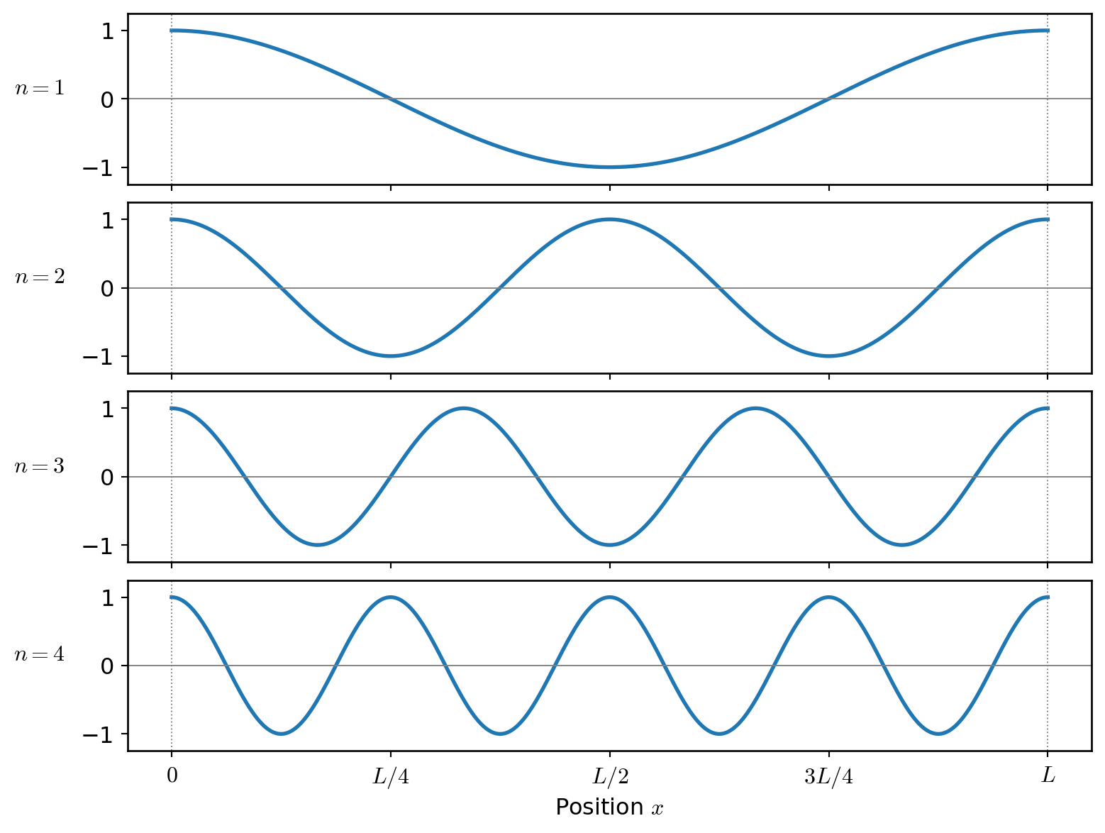
A plane-wave factor \(e^{ikx}\) satisfies this condition only if

\[ e^{ikL}=1, \]

and therefore

\[ \boxed{k_n=\frac{2\pi n}{L},\qquad n\in\mathbb Z.} \]

The integer \(n\) counts the number of complete spatial oscillations across the box. Figure 2 illustrates the real part of several such modes at a fixed time.

import numpy as np
import matplotlib.pyplot as plt

L = 1.0
x = np.linspace(0, L, 800)

fig, axes = plt.subplots(
    4, 1, figsize=(8, 6),
    sharex=True, layout="constrained"
)

for ax, n in zip(axes, range(1,5)):
    ax.plot(x, np.cos(2*np.pi*n*x/L), lw=2)
    ax.axhline(0, color="gray", lw=0.7)
    ax.axvline(0, color="gray", lw=0.7, ls=":")
    ax.axvline(L, color="gray", lw=0.7, ls=":")
    ax.set_ylim(-1.25, 1.25)
    ax.set_yticks([-1, 0, 1])
    ax.set_ylabel(f"$n={n}$", rotation=0, labelpad=22)

axes[-1].set_xticks(
    [0, 0.25, 0.5, 0.75, 1],
    ["$0$", "$L/4$", "$L/2$", "$3L/4$", "$L$"]
)
axes[-1].set_xlabel("Position $x$")

plt.show()

Figure 2: One-dimensional periodic Fourier modes. The integer n counts the number of complete oscillations across the box.

The box is a mathematical convenience, not a physical cavity with reflecting walls. Eventually, we can take the limit \(L\to\infty\).

Extension to three dimensions.

In three dimensions, the allowed wave vectors are

\[ \vec k=\frac{2\pi}{L}(n_x,n_y,n_z), \qquad n_x,n_y,n_z\in\mathbb Z. \]

The Fourier expansion of the vector potential becomes

\[ \vec A(\vec r,t) = \frac{1}{\sqrt V} \sum_{\vec k} \vec A_{\vec k}(t)e^{i\vec k\cdot\vec r}. \]

The wave vector \(\vec k\) determines the spatial variation of each mode. Its direction is perpendicular to surfaces of constant phase, and its magnitude determines the wavelength \(\lambda=2\pi/|\vec k|\).

Transverse polarizations.

The Coulomb-gauge condition places an additional restriction on these Fourier components.

Applying the divergence gives

\[ \vec\nabla\cdot\vec A = \frac{1}{\sqrt V} \sum_{\vec k} i\vec k\cdot\vec A_{\vec k}(t) e^{i\vec k\cdot\vec r}. \]

Because the Fourier functions are linearly independent, the condition \(\vec\nabla\cdot\vec A=0\) requires

\[ \boxed{\vec k\cdot\vec A_{\vec k}(t)=0} \]

for each nonzero \(\vec k\).

Thus, each Fourier amplitude is perpendicular to its wave vector: the electromagnetic field is transverse.

For any nonzero \(\vec k\), there are two independent directions perpendicular to it. We introduce two orthonormal polarization vectors \(\vec\epsilon_{\vec k1}\) and \(\vec\epsilon_{\vec k2}\), satisfying

\[ \boxed{ \vec k\cdot\vec\epsilon_{\vec k\lambda}=0, \qquad \vec\epsilon_{\vec k\lambda}\cdot \vec\epsilon_{\vec k\lambda'} =\delta_{\lambda\lambda'}. } \]

The index \(\lambda=1,2\) labels the two independent transverse polarizations.

We can now express the vector potential as

\[ \boxed{ \vec A(\vec r,t) = \frac{1}{\sqrt V} \sum_{\vec k,\lambda} Q_{\vec k\lambda}(t) \vec\epsilon_{\vec k\lambda} e^{i\vec k\cdot\vec r}. } \]

The vector structure of the field is contained in the polarization vectors, while the coefficients \(Q_{\vec k\lambda}(t)\) describe the time-dependent amplitudes of the individual modes.

Reality condition.

Although complex exponentials are convenient mathematical basis functions, the physical vector potential \(\vec A(\vec r,t)\) must be real.

Since

\[ \left(e^{i\vec k\cdot\vec r}\right)^* =e^{-i\vec k\cdot\vec r}, \]

the Fourier amplitudes at opposite wave vectors must be related. Choosing the same real polarization basis for \(\vec k\) and \(-\vec k\), we obtain

\[ \boxed{ Q_{-\vec k,\lambda} =Q_{\vec k\lambda}^{*}. } \]

Consequently, the coefficients at \(\vec k\) and \(-\vec k\) are not independent.

We will retain the complex Fourier representation because it is convenient for describing traveling waves. When identifying the independent harmonic oscillators, we will simply use the real and imaginary parts of these amplitudes.

In the following, we restrict ourselves to nonzero wave vectors \(\vec k\ne0\), corresponding to the propagating electromagnetic modes.

2.7.4.3. Equations of motion for the normal modes

We now determine how the Fourier amplitudes evolve in time.

Substituting the normal-mode expansion into the electromagnetic wave equation,

\[ \frac{\partial^2\vec A}{\partial t^2} -c^2\nabla^2\vec A=0, \]

we use the fact that

\[ \nabla^2e^{i\vec k\cdot\vec r} =-|\vec k|^2e^{i\vec k\cdot\vec r}. \]

This gives

\[ \sum_{\vec k,\lambda} \left( \ddot Q_{\vec k\lambda} +c^2|\vec k|^2Q_{\vec k\lambda} \right) \vec\epsilon_{\vec k\lambda} e^{i\vec k\cdot\vec r} =0. \]

Because the Fourier modes are linearly independent, the coefficient of each mode must vanish:

\[ \boxed{ \ddot Q_{\vec k\lambda} +\omega_k^2Q_{\vec k\lambda}=0, \qquad \omega_k=c|\vec k|. } \]

This is precisely the equation of motion of a harmonic oscillator.

Each Fourier amplitude evolves independently with frequency \(\omega_k\). The reality condition ensures that the amplitudes at opposite wave vectors remain related.

However, the equation of motion alone does not establish the full equivalence with a mechanical harmonic oscillator. We must also examine the energy of the electromagnetic field.

2.7.4.4. The electromagnetic field as a collection of harmonic oscillators

The energy of the free transverse electromagnetic field is

\[ H_{\mathrm T} = \frac12\int_V \left( \varepsilon_0|\vec E|^2 +\frac{1}{\mu_0}|\vec B|^2 \right)d^3r. \]

Using

\[ \vec E=-\frac{\partial\vec A}{\partial t}, \qquad \vec B=\vec\nabla\times\vec A, \]

and substituting the Fourier expansion, we obtain

\[ \boxed{ H_{\mathrm T} = \frac{\varepsilon_0}{2} \sum_{\vec k,\lambda} \left( |\dot Q_{\vec k\lambda}|^2 +\omega_k^2|Q_{\vec k\lambda}|^2 \right). } \]

NoteDerivation: Field energy in terms of Fourier amplitudes

We start from the normal-mode expansion

\[ \vec A(\vec r,t) = \frac{1}{\sqrt V} \sum_{\vec k,\lambda} Q_{\vec k\lambda}(t) \vec\epsilon_{\vec k\lambda} e^{i\vec k\cdot\vec r}. \]

Electric field energy.

Taking the time derivative gives

\[ \vec E(\vec r,t) = -\frac{1}{\sqrt V} \sum_{\vec k,\lambda} \dot Q_{\vec k\lambda} \vec\epsilon_{\vec k\lambda} e^{i\vec k\cdot\vec r}. \]

Substituting into the electric field energy,

\[ \begin{aligned} U_E &=\frac{\varepsilon_0}{2} \int_V\vec E\cdot\vec E\,d^3r\\ &=\frac{\varepsilon_0}{2V} \sum_{\vec k,\lambda} \sum_{\vec k',\lambda'} \dot Q_{\vec k\lambda} \dot Q_{\vec k'\lambda'} (\vec\epsilon_{\vec k\lambda}\cdot \vec\epsilon_{\vec k'\lambda'}) \int_V e^{i(\vec k+\vec k')\cdot\vec r}\,d^3r. \end{aligned} \]

Periodic boundary conditions give the Fourier orthogonality relation

\[ \frac1V\int_V e^{i(\vec k+\vec k')\cdot\vec r}\,d^3r =\delta_{\vec k',-\vec k}. \]

Thus, only terms with \(\vec k'=-\vec k\) survive. Since the polarization vectors satisfy

\[ \vec\epsilon_{-\vec k,\lambda} =\vec\epsilon_{\vec k,\lambda}, \]

their orthonormality gives

\[ U_E = \frac{\varepsilon_0}{2} \sum_{\vec k,\lambda} \dot Q_{\vec k\lambda} \dot Q_{-\vec k,\lambda}. \]

Using the reality condition

\[ Q_{-\vec k,\lambda}=Q_{\vec k\lambda}^{*}, \]

we obtain

\[ \boxed{ U_E = \frac{\varepsilon_0}{2} \sum_{\vec k,\lambda} |\dot Q_{\vec k\lambda}|^2. } \]

Magnetic field energy.

Taking the curl of the vector potential gives

\[ \begin{aligned} \vec B(\vec r,t) &=\vec\nabla\times\vec A\\ &=\frac{i}{\sqrt V} \sum_{\vec k,\lambda} Q_{\vec k\lambda} (\vec k\times\vec\epsilon_{\vec k\lambda}) e^{i\vec k\cdot\vec r}. \end{aligned} \]

Substituting into the magnetic field energy and using the same Fourier orthogonality relation,

\[ \begin{aligned} U_B &=\frac{1}{2\mu_0} \int_V\vec B\cdot\vec B\,d^3r\\ &=-\frac{1}{2\mu_0} \sum_{\vec k,\lambda,\lambda'} Q_{\vec k\lambda} Q_{-\vec k,\lambda'} (\vec k\times\vec\epsilon_{\vec k\lambda}) \cdot (-\vec k\times\vec\epsilon_{-\vec k,\lambda'}). \end{aligned} \]

The two minus signs cancel.

Using the vector identity

\[ (\vec a\times\vec b)\cdot (\vec a\times\vec c) = |\vec a|^2(\vec b\cdot\vec c) -(\vec a\cdot\vec b)(\vec a\cdot\vec c), \]

together with transversality, we find

\[ (\vec k\times\vec\epsilon_{\vec k\lambda}) \cdot (\vec k\times\vec\epsilon_{\vec k\lambda'}) = |\vec k|^2\delta_{\lambda\lambda'}. \]

Therefore,

\[ U_B = \frac{1}{2\mu_0} \sum_{\vec k,\lambda} |\vec k|^2 Q_{\vec k\lambda}Q_{-\vec k,\lambda}. \]

Using the reality condition and \(1/\mu_0=\varepsilon_0c^2\),

\[ \boxed{ U_B = \frac{\varepsilon_0}{2} \sum_{\vec k,\lambda} \omega_k^2|Q_{\vec k\lambda}|^2. } \]

Total field energy.

Adding the electric and magnetic contributions,

\[ \boxed{ H_{\mathrm T} = \frac{\varepsilon_0}{2} \sum_{\vec k,\lambda} \left( |\dot Q_{\vec k\lambda}|^2 +\omega_k^2|Q_{\vec k\lambda}|^2 \right). } \]

Independent harmonic oscillators.

The energy expression already resembles that of a collection of harmonic oscillators. However, the reality condition

\[ Q_{-\vec k,\lambda}=Q_{\vec k\lambda}^{*} \]

means that the contributions from \(\vec k\) and \(-\vec k\) are equal.

We can therefore restrict the sum to one representative from each pair:

\[ \boxed{ H_{\mathrm T} = \varepsilon_0 \sum_{\vec k>0,\lambda} \left( |\dot Q_{\vec k\lambda}|^2 +\omega_k^2|Q_{\vec k\lambda}|^2 \right). } \]

Here, \(\vec k>0\) is shorthand for selecting exactly one representative from each pair of opposite nonzero wave vectors. It does not imply an ordering of vectors by magnitude.

Each complex amplitude contains two independent real coordinates, which we define as

\[ \boxed{ \begin{aligned} q_{\vec k\lambda}^{(1)} &=\sqrt{2\varepsilon_0}\, \operatorname{Re}Q_{\vec k\lambda},\\ q_{\vec k\lambda}^{(2)} &=\sqrt{2\varepsilon_0}\, \operatorname{Im}Q_{\vec k\lambda}. \end{aligned} } \]

Their corresponding canonical momenta are

\[ p_{\vec k\lambda}^{(1)} =\dot q_{\vec k\lambda}^{(1)}, \qquad p_{\vec k\lambda}^{(2)} =\dot q_{\vec k\lambda}^{(2)}. \]

Using

\[ |Q|^2 =(\operatorname{Re}Q)^2 +(\operatorname{Im}Q)^2, \]

the field energy becomes

\[ \begin{aligned} H_{\mathrm T} =\sum_{\vec k>0,\lambda} \Bigg[ &\frac{(p_{\vec k\lambda}^{(1)})^2}{2} +\frac{\omega_k^2(q_{\vec k\lambda}^{(1)})^2}{2}\\ +&\frac{(p_{\vec k\lambda}^{(2)})^2}{2} +\frac{\omega_k^2(q_{\vec k\lambda}^{(2)})^2}{2} \Bigg]. \end{aligned} \]

Each complex Fourier amplitude therefore corresponds to two independent real harmonic oscillators, associated with its real and imaginary parts.

For simplicity, we can collectively label all independent real oscillators by a single index \(s\). The Hamiltonian then takes the familiar form

\[ \boxed{ H_{\mathrm T} = \sum_s \left( \frac{p_s^2}{2} +\frac{\omega_s^2q_s^2}{2} \right). } \]

We have now established the equivalence at the level of both the equations of motion and the energy:

The free transverse electromagnetic field is mathematically equivalent to an infinite collection of independent harmonic oscillators.

This provides the starting point for quantizing the electromagnetic field. Instead of quantizing the field at every position separately, we can apply the familiar quantum mechanics of the harmonic oscillator to each independent mode.

The complex Fourier representation will remain useful later when we describe photons associated with traveling electromagnetic waves.

2.7.5. Quantization: photons as oscillator excitations

In the previous section, we showed that the free transverse electromagnetic field is mathematically equivalent to a collection of independent harmonic oscillators:

\[ H_{\mathrm T} = \sum_s \left( \frac{p_s^2}{2} +\frac{\omega_s^2q_s^2}{2} \right). \]

We can now quantize these oscillators using exactly the same procedure developed in Section 2.6, The One-Dimensional Quantum Harmonic Oscillator.

We promote the classical coordinates and momenta to operators,

\[ q_s\longrightarrow\hat q_s, \qquad p_s\longrightarrow\hat p_s, \]

and impose the canonical commutation relations

\[ \boxed{ [\hat q_s,\hat p_{s'}] =i\hbar\delta_{ss'}, \qquad [\hat q_s,\hat q_{s'}] =[\hat p_s,\hat p_{s'}]=0. } \]

For each mode, we introduce the annihilation and creation operators

\[ \begin{aligned} \hat a_s &= \sqrt{\frac{\omega_s}{2\hbar}}\hat q_s +\frac{i}{\sqrt{2\hbar\omega_s}}\hat p_s,\\ \hat a_s^\dagger &= \sqrt{\frac{\omega_s}{2\hbar}}\hat q_s -\frac{i}{\sqrt{2\hbar\omega_s}}\hat p_s. \end{aligned} \]

They satisfy

\[ [\hat a_s,\hat a_{s'}^\dagger] =\delta_{ss'}. \]

The Hamiltonian of the electromagnetic field therefore becomes

\[ \boxed{ \hat H_{\mathrm{EM}} = \sum_s\hbar\omega_s \left( \hat a_s^\dagger\hat a_s+\frac12 \right). } \]

Photons and occupation numbers.

We define the number operator for each mode,

\[ \hat N_s=\hat a_s^\dagger\hat a_s, \qquad \hat N_s|n_s\rangle=n_s|n_s\rangle. \]

The energy of a mode containing \(n_s\) excitations is

\[ E_{n_s} = \hbar\omega_s \left(n_s+\frac12\right). \]

The creation operator increases the excitation number by one,

\[ \hat a_s^\dagger|n_s\rangle =\sqrt{n_s+1}|n_s+1\rangle, \]

while the annihilation operator decreases it:

\[ \hat a_s|n_s\rangle =\sqrt{n_s}|n_s-1\rangle. \]

Each excitation carries an energy \(\hbar\omega_s\). We interpret it as one photon in that electromagnetic field mode.

The quantum state of the entire field is specified by the occupation numbers of all modes. A basis of such states is

\[ |n_1,n_2,\ldots\rangle = |n_1\rangle\otimes|n_2\rangle\otimes\cdots. \]

These are called photon number states, or Fock states.

The vacuum state \(|0\rangle\) contains no photons in any mode:

\[ \hat a_s|0\rangle=0 \qquad\text{for every }s. \]

Nevertheless, each mode contributes a zero-point energy \(\hbar\omega_s/2\), giving

\[ \langle0|\hat H_{\mathrm{EM}}|0\rangle = \frac12\sum_s\hbar\omega_s. \]

This sum formally diverges when arbitrarily high-frequency modes are included. In our nonrelativistic treatment, we can set aside this constant energy contribution and concentrate on the observable excitations and fluctuations of the field.

In particular, the vacuum has nonzero electromagnetic field fluctuations, even though it contains no photons.

2.7.5.1. The quantized electromagnetic field

We have quantized the electromagnetic field as a collection of independent harmonic oscillators. However, we have not yet established how their quantum excitations are related to the photons we normally associate with propagating light.

From harmonic oscillators to traveling-wave photons.

Recall that the classical Fourier amplitudes at \(\vec k\) and \(-\vec k\) are related by the reality condition,

\[ Q_{-\vec k,\lambda}=Q_{\vec k\lambda}^*. \]

Each pair therefore corresponds to two independent real oscillators, associated with the cosine and sine components of the electromagnetic field.

Neither component individually describes a wave propagating in a definite direction. However, traveling waves can be constructed by combining these components with an appropriate relative phase:

\[ e^{\pm i\vec k\cdot\vec r} = \cos(\vec k\cdot\vec r) \pm i\sin(\vec k\cdot\vec r). \]

We can make the same transformation at the quantum level. Combining the annihilation operators \(\hat b_1\) and \(\hat b_2\) of the two real oscillators, we define

\[ \boxed{ \hat a_{\vec k\lambda} =\frac{\hat b_1+i\hat b_2}{\sqrt2}, \qquad \hat a_{-\vec k,\lambda} =\frac{\hat b_1-i\hat b_2}{\sqrt2}. } \]

These operators describe photons propagating in opposite directions. They satisfy

\[ \boxed{ [\hat a_{\vec k\lambda}, \hat a_{\vec k'\lambda'}^\dagger] = \delta_{\vec k\vec k'}\delta_{\lambda\lambda'}. } \]

The transformation preserves the Hamiltonian and does not introduce additional degrees of freedom. We have simply chosen a representation in which each photon has a definite propagation direction.

The vector potential operator.

We can now express the electromagnetic field in terms of these traveling-wave photon operators.

The quantized vector potential is

\[ \boxed{ \hat{\vec A}(\vec r) = \sum_{\vec k,\lambda} \sqrt{\frac{\hbar} {2\varepsilon_0\omega_k V}} \vec\epsilon_{\vec k\lambda} \left( \hat a_{\vec k\lambda}e^{i\vec k\cdot\vec r} + \hat a_{\vec k\lambda}^\dagger e^{-i\vec k\cdot\vec r} \right). } \]

Here, we use real polarization vectors, consistent with the classical discussion.

Each annihilation term is accompanied by its Hermitian conjugate. Consequently,

\[ \hat{\vec A}^\dagger(\vec r) = \hat{\vec A}(\vec r), \]

as required for the quantum operator representing the physical vector potential.

The following derivation shows how this expression follows directly from the independent oscillator coordinates introduced in Section 2.7.4.

NoteDerivation: Traveling-wave operators and the quantized vector potential

Consider one pair of opposite wave vectors \(\vec k\) and \(-\vec k\), with a fixed polarization \(\lambda\).

The two independent real oscillator coordinates introduced in Section 2.7.4 are

\[ q^{(1)} =\sqrt{2\varepsilon_0}\operatorname{Re}Q_{\vec k\lambda}, \qquad q^{(2)} =\sqrt{2\varepsilon_0}\operatorname{Im}Q_{\vec k\lambda}. \]

After quantization, their annihilation operators are

\[ \hat b_j = \sqrt{\frac{\omega_k}{2\hbar}}\hat q^{(j)} +\frac{i}{\sqrt{2\hbar\omega_k}}\hat p^{(j)}, \qquad j=1,2. \]

They satisfy

\[ [\hat b_j,\hat b_{j'}^\dagger] =\delta_{jj'}. \]

Defining

\[ \hat a_{\vec k\lambda} =\frac{\hat b_1+i\hat b_2}{\sqrt2}, \qquad \hat a_{-\vec k,\lambda} =\frac{\hat b_1-i\hat b_2}{\sqrt2}, \]

we find that these operators obey the usual bosonic commutation relations.

The transformation also preserves the oscillator Hamiltonian:

\[ \hat b_1^\dagger\hat b_1 +\hat b_2^\dagger\hat b_2 = \hat a_{\vec k\lambda}^\dagger \hat a_{\vec k\lambda} + \hat a_{-\vec k,\lambda}^\dagger \hat a_{-\vec k,\lambda}. \]

Constructing the vector potential.

Recall the classical Fourier amplitude

\[ Q_{\vec k\lambda} = \frac{q^{(1)}+iq^{(2)}} {\sqrt{2\varepsilon_0}}. \]

After quantization,

\[ \hat Q_{\vec k\lambda} = \frac{\hat q^{(1)}+i\hat q^{(2)}} {\sqrt{2\varepsilon_0}}. \]

Using

\[ \hat q^{(j)} = \sqrt{\frac{\hbar}{2\omega_k}} (\hat b_j+\hat b_j^\dagger), \]

we obtain

\[ \boxed{ \hat Q_{\vec k\lambda} = \sqrt{\frac{\hbar}{2\varepsilon_0\omega_k}} \left( \hat a_{\vec k\lambda} +\hat a_{-\vec k,\lambda}^\dagger \right). } \]

The Fourier amplitude at the opposite wave vector is its Hermitian conjugate,

\[ \hat Q_{-\vec k,\lambda} = \hat Q_{\vec k\lambda}^\dagger. \]

Substituting these expressions into

\[ \hat{\vec A}(\vec r) = \frac{1}{\sqrt V} \sum_{\vec k,\lambda} \hat Q_{\vec k\lambda} \vec\epsilon_{\vec k\lambda} e^{i\vec k\cdot\vec r}, \]

and relabeling the wave vectors in the creation-operator terms gives

\[ \boxed{ \hat{\vec A}(\vec r) = \sum_{\vec k,\lambda} \sqrt{\frac{\hbar} {2\varepsilon_0\omega_k V}} \vec\epsilon_{\vec k\lambda} \left( \hat a_{\vec k\lambda}e^{i\vec k\cdot\vec r} + \hat a_{\vec k\lambda}^\dagger e^{-i\vec k\cdot\vec r} \right). } \]

Thus, the traveling-wave expansion follows directly from the quantization of the two independent real oscillators.

The electric field operator.

For the free electromagnetic field, the transverse electric field is related to the vector potential by

\[ \vec E_{\mathrm T} =-\frac{\partial\vec A}{\partial t}. \]

Recall that the momentum of a harmonic oscillator is related to the time derivative of its coordinate, \(p_s=\dot q_s\). After quantization, the momentum operator can be expressed as

\[ \hat p_s = -i\sqrt{\frac{\hbar\omega_s}{2}} (\hat a_s-\hat a_s^\dagger). \]

Using this relation for the independent field oscillators, we obtain the transverse electric field operator

\[ \boxed{ \hat{\vec E}_{\mathrm T}(\vec r) = i\sum_{\vec k,\lambda} \sqrt{\frac{\hbar\omega_k} {2\varepsilon_0 V}} \vec\epsilon_{\vec k\lambda} \left( \hat a_{\vec k\lambda}e^{i\vec k\cdot\vec r} - \hat a_{\vec k\lambda}^\dagger e^{-i\vec k\cdot\vec r} \right). } \]

The electromagnetic field is no longer merely a prescribed function of space and time. Its amplitude is an operator that connects quantum states with different photon numbers.

Because the electric field operator contains both annihilation and creation operators, it can describe processes in which photons are absorbed or emitted by an atom.

2.7.5.2. Vacuum fluctuations and the uncertainty principle

The vacuum contains no photons, but does that mean the electromagnetic field vanishes?

To answer this question, consider a single electromagnetic mode with frequency \(\omega\). At a fixed position, choosing the spatial phase to be zero, the electric field component along its polarization direction can be written

\[ \hat E = iE_0(\hat a-\hat a^\dagger), \qquad E_0= \sqrt{\frac{\hbar\omega} {2\varepsilon_0 V}}. \]

In the vacuum state,

\[ \boxed{ \langle0|\hat E|0\rangle=0. } \]

However, the expectation value of the square of the electric field is not zero:

\[ \boxed{ \langle0|\hat E^2|0\rangle = \frac{\hbar\omega}{2\varepsilon_0 V}. } \]

Since the average field vanishes, this is also its variance:

\[ \boxed{ (\Delta E)^2 = \langle\hat E^2\rangle -\langle\hat E\rangle^2 = \frac{\hbar\omega}{2\varepsilon_0 V}. } \]

Thus, even in the absence of photons, the electric field has nonzero quantum fluctuations.

NoteDerivation: Electric field fluctuations in the vacuum

For a single mode, we write

\[ \hat E=iE_0(\hat a-\hat a^\dagger). \]

Squaring the operator gives

\[ \hat E^2 = -E_0^2 \left( \hat a^2 -\hat a\hat a^\dagger -\hat a^\dagger\hat a +\hat a^{\dagger 2} \right). \]

The vacuum satisfies

\[ \hat a|0\rangle=0. \]

Therefore,

\[ \langle0|\hat a^2|0\rangle = \langle0|\hat a^{\dagger 2}|0\rangle = \langle0|\hat a^\dagger\hat a|0\rangle =0. \]

Using the commutation relation

\[ [\hat a,\hat a^\dagger]=1, \]

we find

\[ \langle0|\hat a\hat a^\dagger|0\rangle=1. \]

Consequently,

\[ \boxed{ \langle0|\hat E^2|0\rangle =E_0^2 =\frac{\hbar\omega}{2\varepsilon_0 V}. } \]

Connection to the uncertainty principle.

These vacuum fluctuations are closely related to the uncertainty principle for a quantum harmonic oscillator.

Recall that the oscillator coordinate and momentum satisfy

\[ \boxed{ \Delta q\,\Delta p\geq\frac{\hbar}{2}. } \]

In classical mechanics, an oscillator can be completely at rest at its equilibrium position, with \(q=p=0\). In quantum mechanics, however, the coordinate and momentum cannot both have precisely defined values.

For the harmonic oscillator ground state,

\[ \langle\hat q\rangle = \langle\hat p\rangle=0, \]

but their variances are nonzero:

\[ (\Delta q)^2=\frac{\hbar}{2\omega}, \qquad (\Delta p)^2=\frac{\hbar\omega}{2}. \]

As we have seen, each independent mode of the electromagnetic field behaves like a quantum harmonic oscillator. The electric field is related to the oscillator momenta, so their quantum uncertainties appear as fluctuations of the electromagnetic field.

The electromagnetic vacuum is therefore not a state in which the electric field has a precisely defined value of zero. Rather, it is the lowest-energy state of the field, with a vanishing average electric field but nonzero fluctuations.

This calculation concerns a single mode. For the full electromagnetic field, the fluctuations involve contributions from all modes, and the field variance at an idealized point requires additional care.

2.7.6. Quantum States of the Electromagnetic Field

Quantizing the electromagnetic field allows us to describe light in terms of photons. However, specifying the number of photons is not the only way to characterize a quantum state of light.

Different quantum states can have very different electric-field properties. In particular, they differ in their average electric field and in the quantum fluctuations around that average.

To visualize these differences, it is useful to introduce a representation based on the two field quadratures.

Field quadratures and the uncertainty principle

Recall that each electromagnetic mode is described by a quantum harmonic oscillator with coordinate \(\hat q\) and momentum \(\hat p\).

For a single mode of frequency \(\omega\), we define the dimensionless quadrature operators

\[ \boxed{ \begin{aligned} \hat X &=\frac{\hat a+\hat a^\dagger}{2} =\sqrt{\frac{\omega}{2\hbar}}\,\hat q,\\[6pt] \hat Y &=\frac{\hat a-\hat a^\dagger}{2i} =\frac{\hat p}{\sqrt{2\hbar\omega}}. \end{aligned} } \]

Thus, the field quadratures are simply rescaled versions of the familiar harmonic oscillator coordinate and momentum.

Since

\[ [\hat q,\hat p]=i\hbar, \]

the quadratures satisfy

\[ [\hat X,\hat Y]=\frac{i}{2}. \]

The position–momentum uncertainty principle therefore becomes

\[ \boxed{ \Delta X\,\Delta Y\geq\frac14. } \]

The quadratures also have a simple connection to the amplitude and phase of an electromagnetic wave.

A classical monochromatic electric field can be written as

\[ E(t)=E_c\cos(\omega t)+E_s\sin(\omega t), \]

or equivalently,

\[ E(t)=E_A\cos(\omega t-\phi), \]

where

\[ E_c=E_A\cos\phi, \qquad E_s=E_A\sin\phi. \]

The two coefficients \(E_c\) and \(E_s\) determine the amplitude \(E_A\) and phase \(\phi\) of the wave.

In the quantum description, the corresponding field components are represented by the operators \(\hat X\) and \(\hat Y\) (up to a choice of phase convention).

We can therefore visualize a quantum state in the \(X\)–\(Y\) plane:

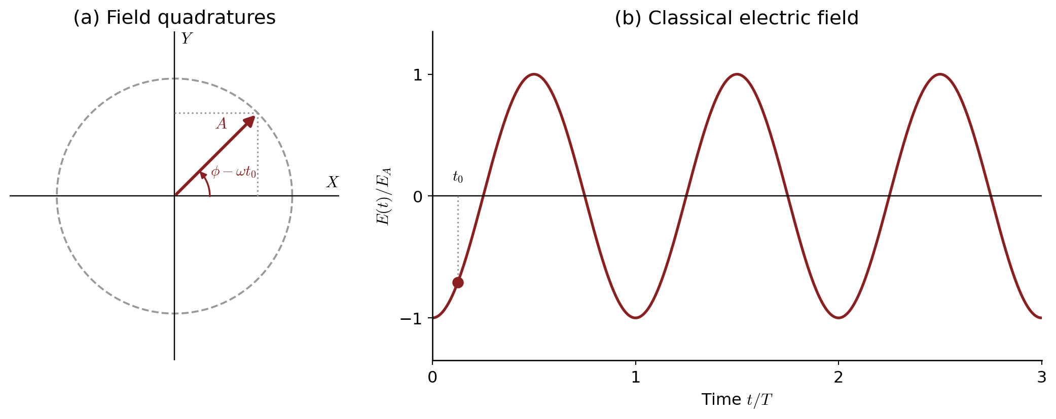
• The mean values \(\langle\hat X\rangle\) and \(\langle\hat Y\rangle\) specify the center of the state’s distribution.
• The distance of this center from the origin is proportional to the mean field amplitude \(E_A\).
• Its angle determines the phase of the mean electromagnetic field. During free evolution, this angle changes as \(\phi-\omega t\).
• The spread around the center represents quantum fluctuations of the field.

The figure below illustrates a classical monochromatic electromagnetic field. Its amplitude and phase are precisely defined, and the field follows a sinusoidal oscillation in time.

import numpy as np
import matplotlib.pyplot as plt

# ------------------------------------------------------------
# Classical monochromatic electromagnetic field
#
# Left:  Quadrature plane (X horizontal, Y vertical)
# Right: Electric field as a function of time
#
# Convention:
#   X(t) = A cos(phi - omega*t)
#   Y(t) = A sin(phi - omega*t)
#   E(t) = -E_A Y(t)/A
#        = E_A sin(omega*t - phi)
# ------------------------------------------------------------

# Parameters
A = 1.0
phi = np.pi / 2
omega = 1.0

T = 2 * np.pi / omega
t0 = T / 8

t = np.linspace(0, 3 * T, 1500)

# Quadratures at the selected instant
theta = phi - omega * t0

X0 = A * np.cos(theta)
Y0 = A * np.sin(theta)

# Normalized electric field
E = np.sin(omega * t - phi)
E0 = np.sin(omega * t0 - phi)

# Colors and styling
red = "#8b1e1e"
gray = "#999999"

plt.rcParams.update({
    "font.size": 12,
    "mathtext.fontset": "cm",
    "axes.linewidth": 1.0,
})

fig, (ax1, ax2) = plt.subplots(
    1, 2,
    figsize=(11, 4.2),
    gridspec_kw={"width_ratios": [1, 1.6]},
    constrained_layout=True
)

# ------------------------------------------------------------
# LEFT: X-Y quadrature plane
# ------------------------------------------------------------

angle = np.linspace(0, 2 * np.pi, 500)

# Circular trajectory
ax1.plot(
    A * np.cos(angle),
    A * np.sin(angle),
    color=gray,
    ls="--",
    lw=1.4
)

# Coordinate axes
ax1.axhline(0, color="black", lw=0.9)
ax1.axvline(0, color="black", lw=0.9)

# Field vector
ax1.annotate(
    "",
    xy=(X0, Y0),
    xytext=(0, 0),
    arrowprops=dict(
        arrowstyle="-|>",
        color=red,
        lw=2.2,
        mutation_scale=16
    )
)

# Projections onto the coordinate axes
ax1.plot(
    [X0, X0], [0, Y0],
    color=gray, ls=":", lw=1.2
)
ax1.plot(
    [0, X0], [Y0, Y0],
    color=gray, ls=":", lw=1.2
)

# Angle arc, measured counterclockwise from +X
r_arc = 0.30 * A
arc = np.linspace(0, theta, 100)

ax1.plot(
    r_arc * np.cos(arc),
    r_arc * np.sin(arc),
    color=red,
    lw=1.3
)

# Arrowhead indicating positive angular direction
dtheta = 0.12

ax1.annotate(
    "",
    xy=(
        r_arc * np.cos(theta),
        r_arc * np.sin(theta)
    ),
    xytext=(
        r_arc * np.cos(theta - dtheta),
        r_arc * np.sin(theta - dtheta)
    ),
    arrowprops=dict(
        arrowstyle="-|>",
        color=red,
        lw=1.2,
        mutation_scale=10
    )
)

# Angle label
ax1.text(
    0.54 * A * np.cos(theta / 2),
    0.54 * A * np.sin(theta / 2),
    r"$\phi-\omega t_0$",
    color=red,
    ha="center",
    va="center",
    fontsize=11
)

# Amplitude label
ax1.text(
    0.65 * X0 - 0.12,
    0.65 * Y0 + 0.12,
    r"$A$",
    color=red
)

ax1.set_xlim(-1.4 * A, 1.4 * A)
ax1.set_ylim(-1.4 * A, 1.4 * A)
ax1.set_aspect("equal")

# Labels at the positive ends of the axes
ax1.text(
    1.34 * A, 0.05 * A,
    r"$X$",
    ha="center",
    va="bottom"
)

ax1.text(
    0.05 * A, 1.34 * A,
    r"$Y$",
    ha="left",
    va="center"
)

ax1.set_title("(a) Field quadratures")

ax1.set_xticks([])
ax1.set_yticks([])

for spine in ax1.spines.values():
    spine.set_visible(False)

# ------------------------------------------------------------
# RIGHT: Electric field versus time
# ------------------------------------------------------------

ax2.plot(
    t / T, E,
    color=red,
    lw=2.0
)

ax2.axhline(0, color="black", lw=0.9)

# Highlight the selected instant t0
ax2.scatter(
    [t0 / T], [E0],
    color=red,
    s=55,
    zorder=5
)

# Dotted projection onto the time axis
ax2.plot(
    [t0 / T, t0 / T],
    [0, E0],
    color=gray,
    ls=":",
    lw=1.2
)

# Label t0 on the time axis
ax2.annotate(
    r"$t_0$",
    xy=(t0 / T, 0),
    xytext=(0, 9),
    textcoords="offset points",
    ha="center",
    va="bottom",
    fontsize=11
)

ax2.set_xlim(0, 3)
ax2.set_ylim(-1.35, 1.35)

ax2.set_xlabel(r"Time $t/T$")
ax2.set_ylabel(r"$E(t)/E_A$")
ax2.set_title("(b) Classical electric field")

ax2.set_xticks([0, 1, 2, 3])
ax2.set_yticks([-1, 0, 1])

ax2.spines["top"].set_visible(False)
ax2.spines["right"].set_visible(False)

plt.show()

Figure 3: Two equivalent representations of a classical monochromatic electromagnetic field. (a) The field quadratures describe a vector of constant amplitude rotating in the X–Y plane. Its angle is measured counterclockwise from the positive X-axis. (b) The corresponding sinusoidal electric field as a function of time. The highlighted point at t₀ corresponds to the vector shown in panel (a).

For a quantum state of the electromagnetic field, the mean values of the quadratures still describe the average field, but quantum fluctuations introduce uncertainty around these values. The uncertainty principle prevents both quadratures from being arbitrarily well defined simultaneously. Different quantum states of light are distinguished by their mean fields and by how these fluctuations are distributed in the \(X\)–\(Y\) plane.

We will use this representation to compare three important types of quantum states of light.

2.7.6.1. Fock states: Light with a definite photon number

A Fock state \(|n\rangle\) contains exactly \(n\) photons in a given electromagnetic mode:

\[ \hat N|n\rangle=n|n\rangle, \qquad \hat N=\hat a^\dagger\hat a. \]

Consequently, its photon-number uncertainty vanishes:

\[ \boxed{ \Delta N=0. } \]

However, a Fock state does not have a nonzero average electric field.

Since the annihilation and creation operators change the photon number,

\[ \langle n|\hat a|n\rangle = \langle n|\hat a^\dagger|n\rangle=0. \]

Therefore,

\[ \boxed{ \langle n|\hat E(t)|n\rangle=0. } \]

This remains true even for a state containing many photons.

The field nevertheless exhibits quantum fluctuations. For the quadratures, we find

\[ \boxed{ (\Delta X)^2 = (\Delta Y)^2 = \frac{2n+1}{4}. } \]

The uncertainties are equal in both directions and increase with photon number.

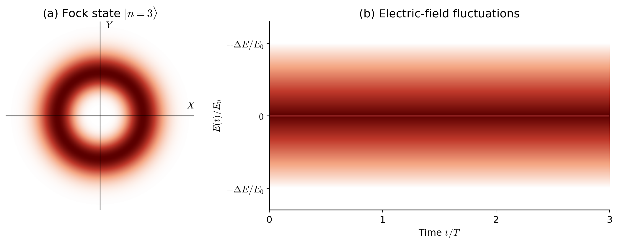
In the \(X\)–\(Y\) plane, Fock states are therefore rotationally symmetric around the origin. They have no preferred optical phase.

The vacuum state \(|0\rangle\) is the simplest example, with

\[ (\Delta X)^2 = (\Delta Y)^2 = \frac14. \]

For \(n>0\), the full phase-space distribution has a more complicated, non-Gaussian structure. Rather than a simple uncertainty circle centered at the origin, it exhibits a ring-like structure, reflecting the absence of a preferred optical phase.

The important distinction is that a Fock state has a precisely defined photon number, but no classical oscillating mean electric field.

import numpy as np
import matplotlib.pyplot as plt
from matplotlib.colors import LinearSegmentedColormap
from math import factorial

# ------------------------------------------------------------
# Fock state |n>
#
# Left:  Husimi Q distribution in the X-Y plane
# Right: Mean electric field and quantum fluctuations
#
# <X> = <Y> = 0
# (Delta X)^2 = (Delta Y)^2 = (2n+1)/4
# <E(t)> = 0
# ------------------------------------------------------------

# Parameters
n = 3
omega = 1.0

T = 2 * np.pi / omega
t = np.linspace(0, 3 * T, 1200)

# Quadrature uncertainty
delta_X = np.sqrt((2 * n + 1) / 4)

# For E(t) = -2 E0 Y(t), the field rms uncertainty is
# Delta E / E0 = 2 Delta Y = sqrt(2n+1).
delta_E = np.sqrt(2 * n + 1)

# Colors
red = "#8b1e1e"
gray = "#999999"

cmap = LinearSegmentedColormap.from_list(
    "field_grad",
    ["#ffffff", "#f4a582", "#c0392b", "#5c0000"]
)

plt.rcParams.update({
    "font.size": 12,
    "mathtext.fontset": "cm",
    "axes.linewidth": 1.0,
})

fig, (ax1, ax2) = plt.subplots(
    1, 2,
    figsize=(11, 4.2),
    gridspec_kw={"width_ratios": [1, 1.6]},
    constrained_layout=True
)

# ------------------------------------------------------------
# LEFT: Husimi Q distribution
# ------------------------------------------------------------

# Coherent-state coordinate alpha = X + iY.
#
# Q_n(alpha) = exp(-|alpha|^2) |alpha|^(2n) / (pi n!)
#
# The maximum occurs at |alpha| = sqrt(n).

limit = 3.8

x = np.linspace(-limit, limit, 550)
y = np.linspace(-limit, limit, 550)

X, Y = np.meshgrid(x, y)
R2 = X**2 + Y**2

Q = np.exp(-R2) * R2**n / (np.pi * factorial(n))
Q /= Q.max()

# Display probability density with white background
ax1.imshow(
    Q,
    extent=[-limit, limit, -limit, limit],
    origin="lower",
    cmap=cmap,
    vmin=0,
    vmax=1,
    interpolation="bilinear"
)

# Coordinate axes
ax1.axhline(0, color="black", lw=0.9, alpha=0.8)
ax1.axvline(0, color="black", lw=0.9, alpha=0.8)

# Axis labels
ax1.text(
    0.96 * limit, 0.06 * limit,
    r"$X$", ha="center", va="bottom"
)
ax1.text(
    0.06 * limit, 0.96 * limit,
    r"$Y$", ha="left", va="center"
)

ax1.set_xlim(-limit, limit)
ax1.set_ylim(-limit, limit)
ax1.set_aspect("equal")

ax1.set_title(rf"(a) Fock state $|n={n}\rangle$")
ax1.set_xticks([])
ax1.set_yticks([])

for spine in ax1.spines.values():
    spine.set_visible(False)

# ------------------------------------------------------------
# RIGHT: Mean electric field and fluctuation band
# ------------------------------------------------------------

# Mean field is zero at all times
E_mean = np.zeros_like(t)

# The band extends to +/- one rms field uncertainty.
# The gradient is darkest at the mean and fades to white
# at the edges, matching the requested visual style.

ny = 500
y_field = np.linspace(
    -1.3 * delta_E,
     1.3 * delta_E,
    ny
)

TT, EE = np.meshgrid(t / T, y_field)

distance = np.abs(EE)

inside = distance <= delta_E
intensity = np.clip(1 - distance / delta_E, 0, 1)

rgba = cmap(intensity)
rgba[..., 3] = np.where(inside, 1.0, 0.0)

ax2.imshow(
    rgba,
    extent=[
        0, 3,
        y_field.min(), y_field.max()
    ],
    origin="lower",
    aspect="auto",
    interpolation="bilinear"
)

# Mean field
ax2.plot(
    t / T,
    E_mean,
    color=red,
    lw=2.0
)

ax2.set_xlim(0, 3)
ax2.set_ylim(-1.3 * delta_E, 1.3 * delta_E)

ax2.set_xlabel(r"Time $t/T$")
ax2.set_ylabel(r"$E(t)/E_0$")
ax2.set_title("(b) Electric-field fluctuations")

ax2.set_xticks([0, 1, 2, 3])
ax2.set_yticks([-delta_E, 0, delta_E])
ax2.set_yticklabels([
    r"$-\Delta E/E_0$",
    "$0$",
    r"$+\Delta E/E_0$"
])

ax2.spines["top"].set_visible(False)
ax2.spines["right"].set_visible(False)

plt.show()

Figure 4: A Fock state with a definite photon number (n = 3). (a) Rotationally symmetric phase-space representation, illustrating the absence of a preferred optical phase. The ring-like distribution reflects the quantum fluctuations of the field. (b) The expectation value of the electric field vanishes at all times, although the field has nonzero quantum fluctuations. The red shading illustrates the rms field uncertainty, which is independent of time.

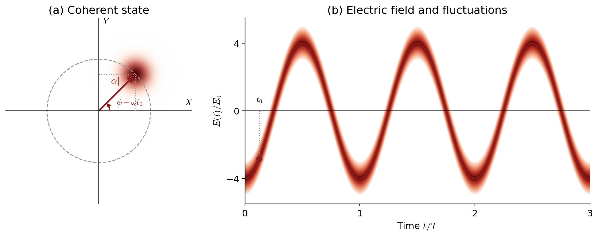
2.7.6.2. Coherent states: The quantum description of classical light

A coherent state \(|\alpha\rangle\) is defined as an eigenstate of the annihilation operator:

\[ \boxed{ \hat a|\alpha\rangle = \alpha|\alpha\rangle, } \]

where \(\alpha\) is a complex number.

Writing

\[ \alpha=|\alpha|e^{i\phi}, \]

we obtain the time-dependent expectation values

\[ \boxed{ \begin{aligned} \langle\hat X\rangle(t) &=|\alpha|\cos(\phi-\omega t),\\ \langle\hat Y\rangle(t) &=|\alpha|\sin(\phi-\omega t). \end{aligned} } \]

Thus, the mean-field vector rotates in the \(X\)–\(Y\) plane at angular frequency \(\omega\), while its distance from the origin remains constant.

Unlike a Fock state, a coherent state therefore has a nonzero mean field amplitude and a well-defined mean optical phase when \(\alpha\ne0\).

For a single mode, the expectation value of the electric field is

\[ \boxed{ \langle\hat E(t)\rangle = 2E_0|\alpha|\sin(\omega t-\phi), } \]

where

\[ E_0= \sqrt{\frac{\hbar\omega}{2\varepsilon_0V}}. \]

Thus, the average electric field oscillates exactly like a classical electromagnetic wave.

However, the photon number is not precisely defined. Instead,

\[ \boxed{ \langle\hat N\rangle=|\alpha|^2, \qquad (\Delta N)^2=|\alpha|^2. } \]

Coherent states have a Poisson distribution of photon numbers. Their relative photon-number uncertainty is

\[ \frac{\Delta N}{\langle\hat N\rangle} = \frac{1}{\sqrt{\langle\hat N\rangle}}. \]

For large photon numbers, this relative uncertainty becomes small.

The quadrature variances are

\[ \boxed{ (\Delta X)^2 = (\Delta Y)^2 = \frac14. } \]

Remarkably, these are exactly the same uncertainties as in the vacuum.

In the \(X\)–\(Y\) plane, a coherent state is therefore represented by a circular Gaussian distribution displaced from the origin.

As the mean photon number increases, the displacement grows while the absolute quadrature uncertainties remain unchanged. The fluctuations therefore become small relative to the mean field amplitude.

This explains why coherent states with large photon occupation numbers provide an excellent quantum description of classical electromagnetic waves.

import numpy as np
import matplotlib.pyplot as plt
from matplotlib.colors import LinearSegmentedColormap

# ------------------------------------------------------------
# Coherent state |alpha>
#
# Left:  Quadrature distribution at t0
# Right: Mean electric field and quantum fluctuations
#
# <X>(t) = |alpha| cos(phi - omega*t)
# <Y>(t) = |alpha| sin(phi - omega*t)
#
# (Delta X)^2 = (Delta Y)^2 = 1/4
#
# <E(t)> / E0 = 2 |alpha| sin(omega*t - phi)
# Delta E / E0 = 1
# ------------------------------------------------------------

# Parameters
alpha_abs = 2.0
phi = np.pi / 2
omega = 1.0

T = 2 * np.pi / omega
t0 = T / 8

t = np.linspace(0, 3 * T, 1500)

theta = phi - omega * t0

X0 = alpha_abs * np.cos(theta)
Y0 = alpha_abs * np.sin(theta)

# Mean electric field and rms uncertainty, in units of E0
E_mean = 2 * alpha_abs * np.sin(omega * t - phi)
E0_mean = 2 * alpha_abs * np.sin(omega * t0 - phi)

delta_X = 0.5
delta_Y = 0.5
delta_E = 1.0

# Colors
red = "#8b1e1e"
gray = "#999999"

cmap = LinearSegmentedColormap.from_list(
    "field_grad",
    ["#ffffff", "#f4a582", "#c0392b", "#5c0000"]
)

plt.rcParams.update({
    "font.size": 12,
    "mathtext.fontset": "cm",
    "axes.linewidth": 1.0,
})

fig, (ax1, ax2) = plt.subplots(
    1, 2,
    figsize=(11, 4.2),
    gridspec_kw={"width_ratios": [1, 1.6]},
    constrained_layout=True
)

# ------------------------------------------------------------
# LEFT: Coherent state in the X-Y plane
# ------------------------------------------------------------

limit = 3.6
grid = np.linspace(-limit, limit, 600)
X, Y = np.meshgrid(grid, grid)

# Circular Gaussian centered on the mean quadratures.
# This is a schematic Gaussian density with standard
# deviations Delta X = Delta Y = 1/2.
density = np.exp(
    -0.5 * (
        ((X - X0) / delta_X)**2
        + ((Y - Y0) / delta_Y)**2
    )
)

# Transparent background outside the Gaussian
rgba = cmap(density)
rgba[..., 3] = np.clip(density, 0, 1)

ax1.imshow(
    rgba,
    extent=[-limit, limit, -limit, limit],
    origin="lower",
    interpolation="bilinear"
)

# Dashed circular trajectory of the mean field
angle = np.linspace(0, 2 * np.pi, 500)

ax1.plot(
    alpha_abs * np.cos(angle),
    alpha_abs * np.sin(angle),
    color=gray,
    ls="--",
    lw=1.2
)

# Coordinate axes
ax1.axhline(0, color="black", lw=0.9)
ax1.axvline(0, color="black", lw=0.9)

# Mean-field vector
ax1.annotate(
    "",
    xy=(X0, Y0),
    xytext=(0, 0),
    arrowprops=dict(
        arrowstyle="-|>",
        color=red,
        lw=2.2,
        mutation_scale=16
    )
)

# Projections onto the coordinate axes
ax1.plot(
    [X0, X0], [0, Y0],
    color=gray, ls=":", lw=1.2
)
ax1.plot(
    [0, X0], [Y0, Y0],
    color=gray, ls=":", lw=1.2
)

# Phase angle, measured counterclockwise from +X
r_arc = 0.42
arc = np.linspace(0, theta, 100)

ax1.plot(
    r_arc * np.cos(arc),
    r_arc * np.sin(arc),
    color=red,
    lw=1.3
)

ax1.annotate(
    "",
    xy=(
        r_arc * np.cos(theta),
        r_arc * np.sin(theta)
    ),
    xytext=(
        r_arc * np.cos(theta - 0.12),
        r_arc * np.sin(theta - 0.12)
    ),
    arrowprops=dict(
        arrowstyle="-|>",
        color=red,
        lw=1.2,
        mutation_scale=10
    )
)

# Phase label
ax1.text(
    0.85 * np.cos(theta / 2) + 0.4,
    0.85 * np.sin(theta / 2),
    r"$\phi-\omega t_0$",
    color=red,
    ha="center",
    va="center",
    fontsize=11
)

# Mean amplitude label
ax1.text(
    0.65 * X0 - 0.55,
    0.65 * Y0 + 0.15,
    r"$|\alpha|$",
    color=red
)

ax1.set_xlim(-limit, limit)
ax1.set_ylim(-limit, limit)
ax1.set_aspect("equal")

# Labels at positive ends of axes
ax1.text(
    0.96 * limit, 0.04 * limit,
    r"$X$",
    ha="center",
    va="bottom"
)

ax1.text(
    0.04 * limit, 0.96 * limit,
    r"$Y$",
    ha="left",
    va="center"
)

ax1.set_title("(a) Coherent state")
ax1.set_xticks([])
ax1.set_yticks([])

for spine in ax1.spines.values():
    spine.set_visible(False)

# ------------------------------------------------------------
# RIGHT: Mean electric field and fluctuation band
# ------------------------------------------------------------

# Gaussian-style gradient within +/- one rms uncertainty.
# The band follows the sinusoidal mean electric field.

ny = 600

y_min = E_mean.min() - 1.5 * delta_E
y_max = E_mean.max() + 1.5 * delta_E

y_field = np.linspace(y_min, y_max, ny)

TT, EE = np.meshgrid(t / T, y_field)

mean_grid = E_mean[np.newaxis, :]

distance = np.abs(EE - mean_grid)

inside = distance <= delta_E
intensity = np.clip(1 - distance / delta_E, 0, 1)

rgba = cmap(intensity)
rgba[..., 3] = np.where(inside, 1.0, 0.0)

ax2.imshow(
    rgba,
    extent=[0, 3, y_min, y_max],
    origin="lower",
    aspect="auto",
    interpolation="bilinear"
)

# Mean electric field
ax2.plot(
    t / T,
    E_mean,
    color=red,
    lw=1.8
)

ax2.axhline(0, color="black", lw=0.8)

# Highlight the instant t0
ax2.scatter(
    [t0 / T],
    [E0_mean],
    color=red,
    s=50,
    zorder=5
)

ax2.plot(
    [t0 / T, t0 / T],
    [0, E0_mean],
    color=gray,
    ls=":",
    lw=1.2
)

ax2.annotate(
    r"$t_0$",
    xy=(t0 / T, 0),
    xytext=(0, 9),
    textcoords="offset points",
    ha="center",
    va="bottom",
    fontsize=11
)

ax2.set_xlim(0, 3)
ax2.set_ylim(y_min, y_max)

ax2.set_xlabel(r"Time $t/T$")
ax2.set_ylabel(r"$E(t)/E_0$")
ax2.set_title("(b) Electric field and fluctuations")

ax2.set_xticks([0, 1, 2, 3])
ax2.set_yticks([
    -2 * alpha_abs,
    0,
    2 * alpha_abs
])

ax2.spines["top"].set_visible(False)
ax2.spines["right"].set_visible(False)

plt.show()

Figure 5: Coherent state of a single electromagnetic mode. (a) The circular Gaussian distribution is displaced from the origin, indicating a nonzero mean field amplitude and a definite mean optical phase. The red vector shows the mean quadratures at time t₀; the shaded region represents quantum fluctuations. (b) The mean electric field oscillates sinusoidally, while the shaded band indicates its rms quantum uncertainty. The fluctuations have the same absolute magnitude as in the vacuum state.

2.7.6.3. Squeezed states: Redistributing quantum uncertainty

The uncertainty principle requires

\[ \Delta X\,\Delta Y\geq\frac14, \]

but it does not require the uncertainties in the two quadratures to be equal.

A squeezed state has reduced fluctuations in one quadrature at the expense of increased fluctuations in the other.

For an appropriately oriented minimum-uncertainty squeezed state, the variances can be written as

\[ \boxed{ (\Delta X)^2=\frac14e^{-2r}, \qquad (\Delta Y)^2=\frac14e^{2r}, } \]

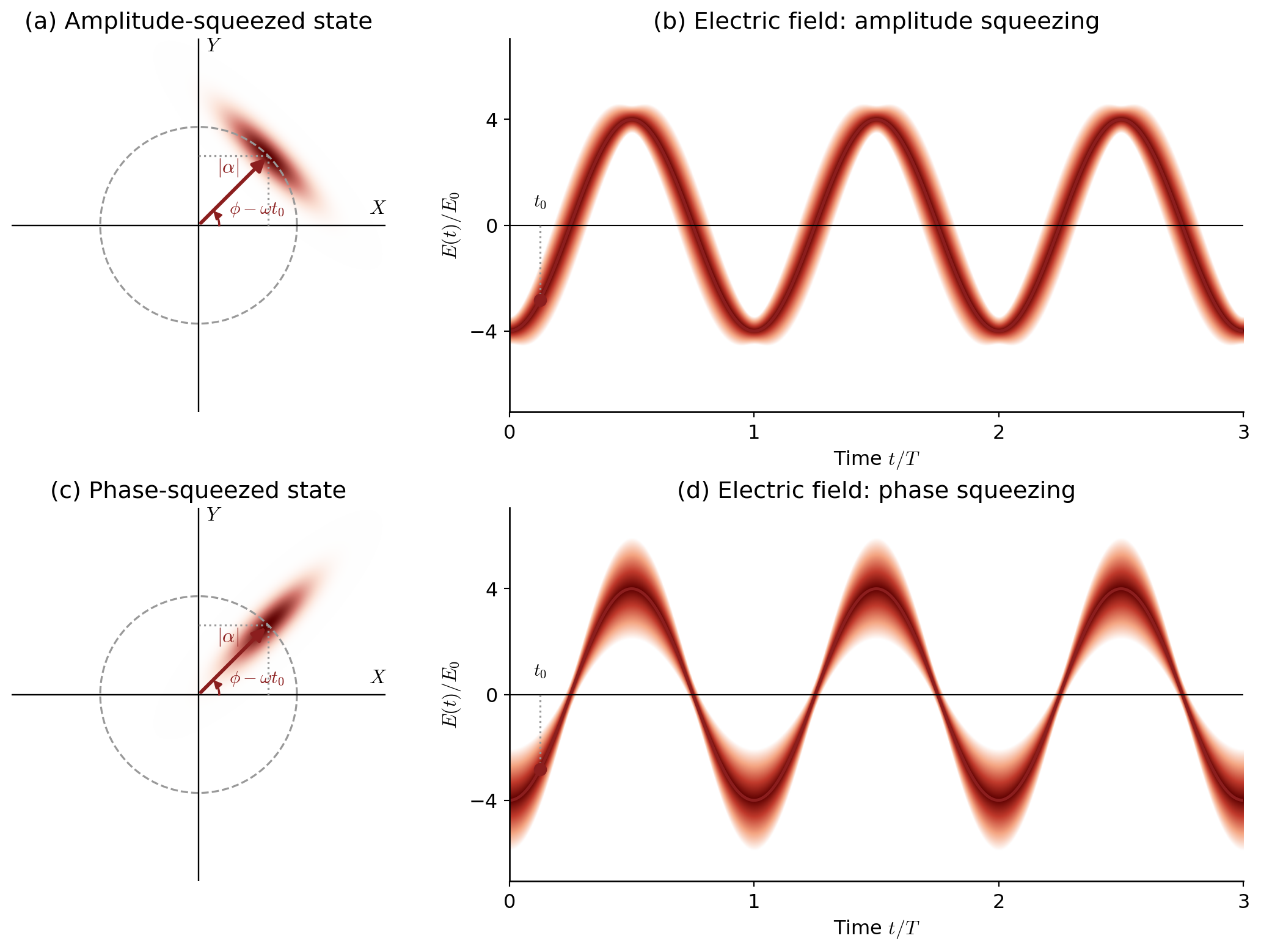
where \(r\geq0\) describes the degree of squeezing.

Their product remains

\[ \Delta X\,\Delta Y=\frac14. \]

The uncertainty principle is therefore not violated. Instead, the quantum fluctuations are redistributed between the two field components.

In the \(X\)–\(Y\) plane, the circular uncertainty region of a coherent state becomes an ellipse.

For a state with a nonzero mean field amplitude, we can distinguish two particularly important cases:

Amplitude-squeezed light.

The uncertainty is reduced along the direction of the mean field amplitude, corresponding to the radial direction in the \(X\)–\(Y\) plane.

The field amplitude becomes more precisely defined, while its phase uncertainty increases.

Phase-squeezed light.

The uncertainty is reduced perpendicular to the mean field amplitude, corresponding to the tangential direction in the \(X\)–\(Y\) plane.

The phase becomes more precisely defined, while the amplitude uncertainty increases.

These descriptions apply most naturally to states with a sufficiently large mean field amplitude, for which radial and angular fluctuations can be interpreted approximately as amplitude and phase noise.

import numpy as np
import matplotlib.pyplot as plt
from matplotlib.colors import LinearSegmentedColormap

# ------------------------------------------------------------
# Squeezed coherent states
#
# Top row:    Amplitude squeezing (radial)
# Bottom row: Phase squeezing (tangential)
#
# X(t) = |alpha| cos(phi - omega*t)
# Y(t) = |alpha| sin(phi - omega*t)
#
# E(t)/E0 = -2 Y(t)
#         = 2 |alpha| sin(omega*t - phi)
#
# Vacuum quadrature uncertainty: Delta X = Delta Y = 1/2
# ------------------------------------------------------------

# Parameters
alpha_abs = 2.0
phi = np.pi / 2
omega = 1.0
r = 0.65

T = 2 * np.pi / omega
t0 = T / 8

t = np.linspace(0, 3 * T, 1500)

theta0 = phi - omega * t0

X0 = alpha_abs * np.cos(theta0)
Y0 = alpha_abs * np.sin(theta0)

# Mean electric field, normalized to E0
E_mean = 2 * alpha_abs * np.sin(omega * t - phi)
E_at_t0 = 2 * alpha_abs * np.sin(omega * t0 - phi)

# Radial and tangential unit vectors at t0
u_r = np.array([np.cos(theta0), np.sin(theta0)])
u_t = np.array([-np.sin(theta0), np.cos(theta0)])

# Minimum-uncertainty squeezed quadrature standard deviations
sigma_small = 0.5 * np.exp(-r)
sigma_large = 0.5 * np.exp(r)

# Colors
red = "#8b1e1e"
gray = "#999999"

cmap = LinearSegmentedColormap.from_list(
    "field_grad",
    ["#ffffff", "#f4a582", "#c0392b", "#5c0000"]
)

plt.rcParams.update({
    "font.size": 12,
    "mathtext.fontset": "cm",
    "axes.linewidth": 1.0,
})

fig, axes = plt.subplots(
    2, 2,
    figsize=(11, 8),
    gridspec_kw={"width_ratios": [1, 1.6]},
    constrained_layout=True
)

# ------------------------------------------------------------
# Helper: X-Y phase-space panel
# ------------------------------------------------------------

def plot_phase_space(ax, sigma_radial, sigma_tangential, title):

    limit = 3.8
    grid = np.linspace(-limit, limit, 600)
    X, Y = np.meshgrid(grid, grid)

    dx = X - X0
    dy = Y - Y0

    # Coordinates relative to radial and tangential directions
    radial = dx * u_r[0] + dy * u_r[1]
    tangential = dx * u_t[0] + dy * u_t[1]

    # Elliptical Gaussian visualization
    density = np.exp(
        -0.5 * (
            (radial / sigma_radial)**2
            + (tangential / sigma_tangential)**2
        )
    )

    rgba = cmap(density)
    rgba[..., 3] = np.clip(density, 0, 1)

    ax.imshow(
        rgba,
        extent=[-limit, limit, -limit, limit],
        origin="lower",
        interpolation="bilinear"
    )

    # Circular trajectory of the mean-field vector
    angle = np.linspace(0, 2 * np.pi, 500)

    ax.plot(
        alpha_abs * np.cos(angle),
        alpha_abs * np.sin(angle),
        color=gray,
        ls="--",
        lw=1.2
    )

    # Coordinate axes
    ax.axhline(0, color="black", lw=0.9)
    ax.axvline(0, color="black", lw=0.9)

    # Mean-field vector
    ax.annotate(
        "",
        xy=(X0, Y0),
        xytext=(0, 0),
        arrowprops=dict(
            arrowstyle="-|>",
            color=red,
            lw=2.2,
            mutation_scale=16
        )
    )

    # Quadrature projections
    ax.plot(
        [X0, X0], [0, Y0],
        color=gray, ls=":", lw=1.2
    )
    ax.plot(
        [0, X0], [Y0, Y0],
        color=gray, ls=":", lw=1.2
    )

    # Phase angle measured counterclockwise from +X
    r_arc = 0.42
    arc = np.linspace(0, theta0, 100)

    ax.plot(
        r_arc * np.cos(arc),
        r_arc * np.sin(arc),
        color=red,
        lw=1.3
    )

    ax.annotate(
        "",
        xy=(
            r_arc * np.cos(theta0),
            r_arc * np.sin(theta0)
        ),
        xytext=(
            r_arc * np.cos(theta0 - 0.12),
            r_arc * np.sin(theta0 - 0.12)
        ),
        arrowprops=dict(
            arrowstyle="-|>",
            color=red,
            lw=1.2,
            mutation_scale=10
        )
    )

    ax.text(
        0.85 * np.cos(theta0 / 2) + 0.4,
        0.85 * np.sin(theta0 / 2),
        r"$\phi-\omega t_0$",
        color=red,
        ha="center",
        va="center",
        fontsize=11
    )

    # Amplitude label
    ax.text(
        0.65 * X0 - 0.55,
        0.65 * Y0 + 0.15,
        r"$|\alpha|$",
        color=red
    )

    # Coordinate-axis labels
    ax.text(
        0.96 * limit, 0.04 * limit,
        r"$X$",
        ha="center",
        va="bottom"
    )

    ax.text(
        0.04 * limit, 0.96 * limit,
        r"$Y$",
        ha="left",
        va="center"
    )

    ax.set_xlim(-limit, limit)
    ax.set_ylim(-limit, limit)
    ax.set_aspect("equal")

    ax.set_title(title)
    ax.set_xticks([])
    ax.set_yticks([])

    for spine in ax.spines.values():
        spine.set_visible(False)


# ------------------------------------------------------------
# Helper: Time-dependent electric-field panel
# ------------------------------------------------------------

def plot_electric_field(ax, squeezing_type, title):

    # The squeezing ellipse rotates with the mean field.
    # Its projection onto the Y quadrature determines
    # the instantaneous electric-field uncertainty.

    theta = phi - omega * t

    if squeezing_type == "amplitude":
        sigma_r = sigma_small
        sigma_t = sigma_large
    else:
        sigma_r = sigma_large
        sigma_t = sigma_small

    # Variance of the Y projection:
    #
    # Delta Y^2(t) =
    #   sigma_r^2 sin^2(theta)
    # + sigma_t^2 cos^2(theta)
    #
    # Since E/E0 = -2Y:
    # Delta E/E0 = 2 Delta Y

    delta_E = 2 * np.sqrt(
        sigma_r**2 * np.sin(theta)**2
        + sigma_t**2 * np.cos(theta)**2
    )

    ny = 650

    y_min = E_mean.min() - 1.6 * delta_E.max()
    y_max = E_mean.max() + 1.6 * delta_E.max()

    y_field = np.linspace(y_min, y_max, ny)

    TT, EE = np.meshgrid(t / T, y_field)

    mean_grid = E_mean[np.newaxis, :]
    width_grid = delta_E[np.newaxis, :]

    distance = np.abs(EE - mean_grid)

    inside = distance <= width_grid
    intensity = np.clip(
        1 - distance / width_grid,
        0, 1
    )

    rgba = cmap(intensity)
    rgba[..., 3] = np.where(inside, 1.0, 0.0)

    ax.imshow(
        rgba,
        extent=[0, 3, y_min, y_max],
        origin="lower",
        aspect="auto",
        interpolation="bilinear"
    )

    # Mean electric field
    ax.plot(
        t / T,
        E_mean,
        color=red,
        lw=1.8
    )

    ax.axhline(0, color="black", lw=0.8)

    # Highlight t0
    ax.scatter(
        [t0 / T],
        [E_at_t0],
        color=red,
        s=50,
        zorder=5
    )

    ax.plot(
        [t0 / T, t0 / T],
        [0, E_at_t0],
        color=gray,
        ls=":",
        lw=1.2
    )

    ax.annotate(
        r"$t_0$",
        xy=(t0 / T, 0),
        xytext=(0, 9),
        textcoords="offset points",
        ha="center",
        va="bottom",
        fontsize=11
    )

    ax.set_xlim(0, 3)
    ax.set_ylim(y_min, y_max)

    ax.set_xlabel(r"Time $t/T$")
    ax.set_ylabel(r"$E(t)/E_0$")
    ax.set_title(title)

    ax.set_xticks([0, 1, 2, 3])
    ax.set_yticks([-2 * alpha_abs, 0, 2 * alpha_abs])

    ax.spines["top"].set_visible(False)
    ax.spines["right"].set_visible(False)


# ------------------------------------------------------------
# TOP ROW: Amplitude-squeezed coherent state
# ------------------------------------------------------------

plot_phase_space(
    axes[0, 0],
    sigma_radial=sigma_small,
    sigma_tangential=sigma_large,
    title="(a) Amplitude-squeezed state"
)

plot_electric_field(
    axes[0, 1],
    squeezing_type="amplitude",
    title="(b) Electric field: amplitude squeezing"
)

# ------------------------------------------------------------
# BOTTOM ROW: Phase-squeezed coherent state
# ------------------------------------------------------------

plot_phase_space(
    axes[1, 0],
    sigma_radial=sigma_large,
    sigma_tangential=sigma_small,
    title="(c) Phase-squeezed state"
)

plot_electric_field(
    axes[1, 1],
    squeezing_type="phase",
    title="(d) Electric field: phase squeezing"
)

plt.show()

Figure 6: Amplitude- and phase-squeezed coherent states of a single electromagnetic mode. Top row: amplitude squeezing reduces fluctuations along the mean-field vector, producing an uncertainty ellipse elongated in the tangential direction. The electric-field uncertainty is smallest near the extrema of the mean oscillation. Bottom row: phase squeezing reduces fluctuations perpendicular to the mean-field vector, producing a radially elongated ellipse. The electric-field uncertainty is smallest near the zero crossings. Both states have the same mean electric field, and neither violates the uncertainty principle.

Squeezed states illustrate an important feature of quantum light: the fluctuations of the electromagnetic field are not necessarily fixed at the vacuum level. They can be redistributed, allowing one field component to be measured with reduced quantum uncertainty.

TipPhysical interpretation

A photon is not a small classical wave packet attached to a point in space. It is a quantum excitation of an electromagnetic mode.

The mode specifies the spatial structure, frequency, and polarization of the field. The quantum state determines its photon occupation and the statistical properties of its electric field.

Fock states, coherent states, and squeezed states are different quantum states of the same electromagnetic mode.

2.7.8. Summary

The route from classical electrodynamics to the quantum description of light can now be summarized:

1. The Lorentz force follows from a Lagrangian containing the scalar and vector potentials.
2. The canonical momentum \(\vec p=m\vec v+q\vec A\) leads to the minimal-coupling Hamiltonian, which describes the interaction between charged particles and electromagnetic fields.
3. In Coulomb gauge, the longitudinal electric field accounts for electrostatic interactions, while the transverse field contains the independent radiation degrees of freedom.
4. Each transverse electromagnetic mode behaves as a harmonic oscillator. Quantizing these oscillators introduces photon creation and annihilation operators, with photons representing discrete excitations of the field modes.
5. Even in the vacuum state, the electromagnetic field exhibits quantum fluctuations, reflecting the uncertainty principle and the nonzero ground-state energy of each mode.
6. Different quantum states describe different properties of light: Fock states have a definite photon number, coherent states most closely resemble classical electromagnetic waves, and squeezed states redistribute quantum uncertainty between field quadratures.

The central result is that light is a quantum field whose excitations are photons. Classical electromagnetic waves emerge from suitable quantum states of this field, particularly coherent states with large mean photon numbers.

Further reading. C. Cohen-Tannoudji, B. Diu, and F. Laloë, Quantum Mechanics, Vol. III, Chapter XVIII, especially the discussion of transverse fields and normal variables. The present exposition uses real oscillator coordinates to identify the independent degrees of freedom before introducing traveling-wave photon modes and their quantum states.